ClickHouse Release 25.1

Another month goes by, which means it’s time for another release!

ClickHouse version 25.1 contains 15 new features 🦃 36 performance optimizations ⛸️ 77 bug fixes 🏕️

In this release, we’ve accelerated the parallel hash join algorithm using a two-level hash map, introduced MinMax indices at the table level, improved Merge tables, added auto-increment functionality, and more!

A special welcome to all the new contributors in 25.1! The growth of ClickHouse's community is humbling, and we are always grateful for the contributions that have made ClickHouse so popular.

Below are the names of the new contributors:

Artem Yurov, Gamezardashvili George, Garrett Thomas, Ivan Nesterov, Jesse Grodman, Jony Mohajan, Juan A. Pedreira, Julian Meyers, Kai Zhu, Manish Gill, Michael Anastasakis, Olli Draese, Pete Hampton, RinChanNOWWW, Sameer Tamsekar, Sante Allegrini, Sergey, Vladimir Zhirov, Yutong Xiao, heymind, jonymohajanGmail, mkalfon, ollidraese

Hint: if you’re curious how we generate this list… here.

You can also view the slides from the presentation.

The parallel hash join has been the default join strategy since version 24.11 and was already ClickHouse’s fastest in-memory hash table join algorithm. Yet, as promised, we keep pushing join performance further in every release with meticulous low-level optimizations.

In version 24.7, we improved the hash table allocation for the parallel hash join. Since version 24.12, ClickHouse can automatically determine which table in the join query should be used for the parallel hash join’s build phase. In 25.1, we’ve also sped up the algorithm's probe phase.

To understand this improvement, let’s first briefly explain how the build phase and probe phase previously worked. This diagram illustrates the previous mechanics of the parallel hash join in ClickHouse (click to enlarge):

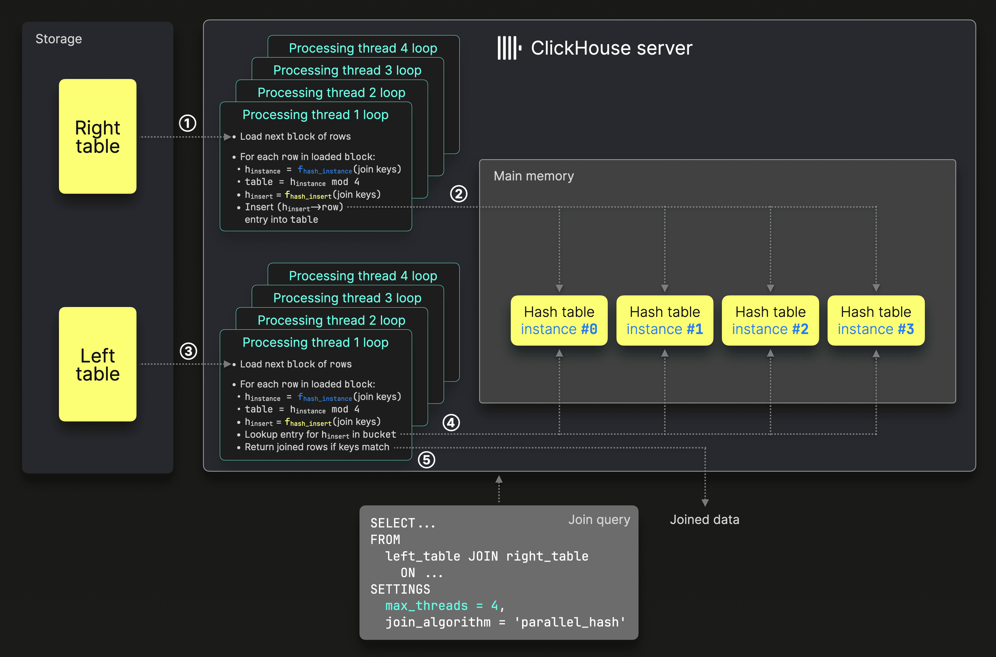
In the algorithm’s ① build phase, the data from the right table is split and processed in parallel by N processing threads to fill N hash table instances in parallel. N is controlled by the max_threads setting, which is 4 in our example. Each processing thread runs a loop:

1. Load the next unprocessed block of rows from the right table.
2. Apply an instance hash function (blue in the diagram) to the join keys of each row, then take the result modulo the number of threads to determine the target hash table instance.
3. Apply an insert hash function (yellow in the diagram) to the join keys and use the result as the key to ② insert the row data into the selected hash table instance.
4. Repeat from Step 1.

In the algorithm’s ③ probe phase, data from the left table is split and processed in parallel by N processing threads (again, N is controlled by the max_threads setting). Each processing thread runs a loop:

1. Load the next unprocessed block of rows from the left table.
2. Apply the same instance hash function used in the build phase (blue in the diagram) to the join keys of each row, then take the result modulo the number of threads to determine the lookup hash table instance.
3. Apply the same insert hash function used in the build phase (yellow in the diagram) to the join keys and use the result to perform a ④ lookup in the selected hash table instance.
4. If the lookup succeeds and the join key values match, ⑤ return the joined rows.
5. Repeat from Step 1.

The parallel hash join’s build phase described above speeds up processing by concurrently filling multiple hash tables, making it faster than the non-parallel hash join, which relies on a single hash table.

Since hash tables are not thread-safe for concurrent inserts, the non-parallel hash join performs all insertions on a single thread, which can become a bottleneck for larger tables in join queries. However, hash tables are thread-safe for concurrent reads, allowing the probe phase in the non-parallel hash join to read from a single hash table in parallel efficiently.

In contrast, the parallel hash join’s concurrent build phase introduces overhead in the above-described probe phase, as input blocks from the left table must first be split and routed to the appropriate hash table instances.

To address this, the probe phase now uses a single shared hash table that all processing threads can access concurrently, just like in the non-parallel hash join. This eliminates the need for input block splitting, reduces overhead, and improves efficiency.

The next diagram illustrates the improved mechanics of the parallel hash join in ClickHouse (click to enlarge):

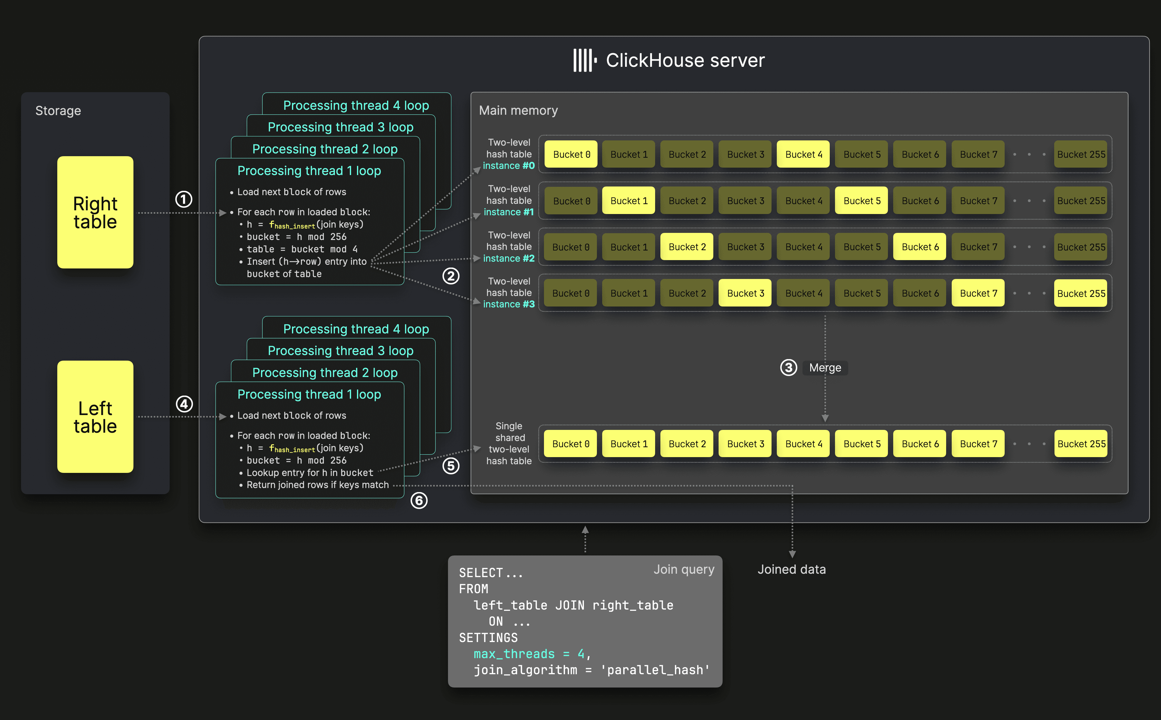
The ① build phase is still executed concurrently. However, when max_threads is set to N, instead of filling N separate hash table instances in parallel, the process now uses N two-level hash table instances. Their 256 buckets are filled concurrently by N processing threads, but in a non-overlapping manner:

• for hash table instance #0, the threads only fill bucket #0, bucket #N, bucket #(N * 2), …
• for hash table instance #1, the threads only fill bucket #1, bucket #N + 1, bucket #(N * 2 + 1), …
• for hash table instance #2, the threads only fill bucket #2, bucket #N + 2, bucket #(N * 2 + 2), …
• for hash table instance #3, the threads only fill bucket #3, bucket #N + 3, bucket #(N * 2 + 3), …
• and so on…

To achieve this, each processing thread runs a loop:

1. Load the next unprocessed block of rows from the right table.
2. Apply an insert hash function (yellow in the diagram) to the join keys of each row, then take the result modulo 256 to determine the target bucket number.
3. Take the target bucket number from step 2 modulo the number of threads to determine the target two-level hash table instance.
4. Use the result of the insert hash function from step 1 as the key to ② insert the row data into the selected bucket number of the selected two-level hash table instance.
5. Repeat from Step 1.

Filling the buckets of the N two-level hash table instances without overlap during the build phase enables efficient (constant-time) ③ merging of these N instances into a single shared two-level hash table. This is efficient because merging simply involves placing all filled buckets into a new two-level hash table container without the need to combine entries across buckets.

In the ④ probe phase, all N processing threads can then read from this shared two-level hash table concurrently, just like in the non-parallel hash join. Each processing thread runs a loop:

1. Load the next unprocessed block of rows from the left table.
2. Apply the same insert hash function used in the build phase (yellow in the diagram) to the join keys of each row, then take the result modulo 256 to determine the bucket number for the lookup in the shared two-level hash table.
3. Perform a ⑤ lookup in the selected bucket.
4. If the lookup succeeds and the join key values match, ⑥ return the joined rows.
5. Repeat from Step 1.

Note that compared to the previous implementation, only a single hash function is now used in both the build and probe phases instead of two. The indirection introduced by the two-level hash table requires only lightweight modulo operations.

To showcase the new parallel hash join's speed improvements, we first run a synthetic test on an AWS EC2 m6i.8xlarge instance with 32 vCPUs and 128 GiB RAM.

We run this query on ClickHouse version 24.12:

1SELECT
2    count(c),
3    version()
4FROM numbers_mt(100000000) AS a
5INNER JOIN
6(
7    SELECT
8        number,
9        toString(number) AS c
10    FROM numbers(2000000)
11) AS b ON (a.number % 10000000) = b.number
12SETTINGS join_algorithm = 'parallel_hash';

   ┌─count(c)─┬─version()──┐
1. │ 20000000 │ 24.12.1.27 │
   └──────────┴────────────┘

1 row in set. Elapsed: 0.521 sec. Processed 102.00 million rows, 816.00 MB (195.83 million rows/s., 1.57 GB/s.)
Peak memory usage: 259.52 MiB.

And on ClickHouse version 25.1:

1SELECT
2    count(c),
3    version()
4FROM numbers_mt(100000000) AS a
5INNER JOIN
6(
7    SELECT
8        number,
9        toString(number) AS c
10    FROM numbers(2000000)
11) AS b ON (a.number % 10000000) = b.number
12SETTINGS join_algorithm = 'parallel_hash';

   ┌─count(c)─┬─version()─┐
1. │ 20000000 │ 25.1.3.23 │
   └──────────┴───────────┘

1 row in set. Elapsed: 0.330 sec. Processed 102.00 million rows, 816.00 MB (309.09 million rows/s., 2.47 GB/s.)
Peak memory usage: 284.96 MiB.

0.330 seconds is approximately 36.66% faster than 0.521 seconds.

Speed improvements are also tested on the same machine using the TPC-H dataset with a scaling factor of 100. The tables, modeling a wholesale supplier’s data warehouse, were created and loaded following the official documentation.

A typical query joins the lineitem and orders tables using ClickHouse 24.12. The hot run results are shown below, where the hot run is the fastest of three consecutive runs:

1SELECT
2    count(),
3    version()
4FROM lineitem AS li
5INNER JOIN orders AS o ON li.l_partkey = o.o_orderkey
6SETTINGS join_algorithm = 'parallel_hash';

   ┌───count()─┬─version()──┐
1. │ 150007337 │ 24.12.1.27 │
   └───────────┴────────────┘

1 row in set. Elapsed: 4.104 sec. Processed 750.04 million rows, 3.00 GB (182.77 million rows/s., 731.10 MB/s.)
Peak memory usage: 16.42 GiB.

Now on ClickHouse version 25.1:

1SELECT
2    count(),
3    version()
4FROM lineitem AS li
5INNER JOIN orders AS o ON li.l_partkey = o.o_orderkey
6SETTINGS join_algorithm = 'parallel_hash';

   ┌───count()─┬─version()─┐
1. │ 150007337 │ 25.1.3.23 │
   └───────────┴───────────┘

1 row in set. Elapsed: 3.056 sec. Processed 750.04 million rows, 3.00 GB (245.42 million rows/s., 981.67 MB/s.)
Peak memory usage: 16.19 GiB.

3.056 seconds is approximately 25.54% faster than 4.104 seconds.

Stay tuned for even more join performance improvements in the next release—and the ones after that (you get the idea)!

The MinMax index stores the minimum and maximum values of the index expression for each block. It’s useful for columns where the data is somewhat sorted - it will not be effective if the data is completely random.

Before the 25.1 release, we needed to specify this index type for each column individually. 25.1 introduces the add_minmax_index_for_numeric_columns setting, which applies the index to all numeric columns.

Let’s learn how to use this setting with the StackOverflow dataset, which contains over 50 million questions, answers, tags, and more. We’ll create a database called stackoverflow:

1CREATE DATABASE stackoverflow;

A create table statement without the MinMax index applied is shown below:

1CREATE TABLE stackoverflow.posts
2(
3    `Id` Int32 CODEC(Delta(4), ZSTD(1)),
4    `PostTypeId` Enum8('Question' = 1, 'Answer' = 2, 'Wiki' = 3, 'TagWikiExcerpt' = 4, 'TagWiki' = 5, 'ModeratorNomination' = 6, 'WikiPlaceholder' = 7, 'PrivilegeWiki' = 8),
5    `AcceptedAnswerId` UInt32,
6    `CreationDate` DateTime64(3, 'UTC'),
7    `Score` Int32,
8    `ViewCount` UInt32 CODEC(Delta(4), ZSTD(1)),
9    `Body` String,
10    `OwnerUserId` Int32,
11    `OwnerDisplayName` String,
12    `LastEditorUserId` Int32,
13    `LastEditorDisplayName` String,
14    `LastEditDate` DateTime64(3, 'UTC') CODEC(Delta(8), ZSTD(1)),
15    `LastActivityDate` DateTime64(3, 'UTC'),
16    `Title` String,
17    `Tags` String,
18    `AnswerCount` UInt16 CODEC(Delta(2), ZSTD(1)),
19    `CommentCount` UInt8,
20    `FavoriteCount` UInt8,
21    `ContentLicense` LowCardinality(String),
22    `ParentId` String,
23    `CommunityOwnedDate` DateTime64(3, 'UTC'),
24    `ClosedDate` DateTime64(3, 'UTC')
25)
26ENGINE = MergeTree
27ORDER BY (PostTypeId, toDate(CreationDate), CreationDate);

Now for one that has the MinMax index applied to all columns.

1CREATE TABLE stackoverflow.posts_min_max
2(
3   `Id` Int32 CODEC(Delta(4), ZSTD(1)),
4   `PostTypeId` Enum8('Question' = 1, 'Answer' = 2, 'Wiki' = 3, 'TagWikiExcerpt' = 4, 'TagWiki' = 5, 'ModeratorNomination' = 6, 'WikiPlaceholder' = 7, 'PrivilegeWiki' = 8),
5   `AcceptedAnswerId` UInt32,
6   `CreationDate` DateTime64(3, 'UTC'),
7   `Score` Int32,
8   `ViewCount` UInt32 CODEC(Delta(4), ZSTD(1)),
9   `Body` String,
10   `OwnerUserId` Int32,
11   `OwnerDisplayName` String,
12   `LastEditorUserId` Int32,
13   `LastEditorDisplayName` String,
14   `LastEditDate` DateTime64(3, 'UTC') CODEC(Delta(8), ZSTD(1)),
15   `LastActivityDate` DateTime64(3, 'UTC'),
16   `Title` String,
17   `Tags` String,
18   `AnswerCount` UInt16 CODEC(Delta(2), ZSTD(1)),
19   `CommentCount` UInt8,
20   `FavoriteCount` UInt8,
21   `ContentLicense` LowCardinality(String),
22   `ParentId` String,
23   `CommunityOwnedDate` DateTime64(3, 'UTC'),
24   `ClosedDate` DateTime64(3, 'UTC')
25)
26ENGINE = MergeTree
27PRIMARY KEY (PostTypeId, toDate(CreationDate), CreationDate)
28ORDER BY (PostTypeId, toDate(CreationDate), CreationDate, CommentCount)
29SETTINGS add_minmax_index_for_numeric_columns=1;

In the first table, the primary key was the same as the sorting key (the primary key defaults to the sorting key when not provided). We’ll have the same primary key in this table, but we’ve added CommentCount to the sorting key to make the MinMax index more effective.

We can write more efficient queries that filter on the CommentCount and against FavoriteCount and AnswerCount, which correlate with CommentCount.

We can check that the MinMax index has been created on all numeric fields by running the following query:

1SELECT name, type, granularity
2FROM system.data_skipping_indices
3WHERE (database = 'stackoverflow') AND (`table` = 'posts_min_max');

┌─name───────────────────────────────┬─type───┬─granularity─┐
│ auto_minmax_index_Id               │ minmax │           1 │
│ auto_minmax_index_AcceptedAnswerId │ minmax │           1 │
│ auto_minmax_index_Score            │ minmax │           1 │
│ auto_minmax_index_ViewCount        │ minmax │           1 │
│ auto_minmax_index_OwnerUserId      │ minmax │           1 │
│ auto_minmax_index_LastEditorUserId │ minmax │           1 │
│ auto_minmax_index_AnswerCount      │ minmax │           1 │
│ auto_minmax_index_CommentCount     │ minmax │           1 │
│ auto_minmax_index_FavoriteCount    │ minmax │           1 │
└────────────────────────────────────┴────────┴─────────────┘

A granularity value of 1 tells us that ClickHouse is creating a MinMax index for each column for each granule.

It’s time to insert data into both tables, starting with posts:

1INSERT INTO stackoverflow.posts 
2SELECT * 
3FROM s3('https://datasets-documentation.s3.eu-west-3.amazonaws.com/stackoverflow/parquet/posts/*.parquet');

We’ll then read the data from posts into posts_min_max:

1INSERT INTO stackoverflow.posts_min_max
2SELECT *
3FROM stackoverflow.posts;

Once that’s done, let’s write a query against each table. This query returns the questions with more than 50 comments and more than 10,000 views:

1FROM stackoverflow.posts
2WHERE PostTypeId = 'Question'
3AND CommentCount > 50 AND ViewCount > 10000;

1SELECT Id, ViewCount, CommentCount
2FROM stackoverflow.posts_min_max
3WHERE PostTypeId = 'Question'
4AND CommentCount > 50 AND ViewCount > 10000;

The results of running this query are shown below:

┌───────Id─┬─ViewCount─┬─CommentCount─┐
│ 44796613 │     40560 │           61 │
│  3538156 │     89863 │           57 │
│ 33762339 │     12104 │           55 │
│  5797014 │     82433 │           55 │
│ 37629745 │     43433 │           89 │
│ 16209819 │     12343 │           54 │
│ 57726401 │     23950 │           51 │
│ 24203940 │     11403 │           56 │
│ 43343231 │     32926 │           51 │
│ 48729384 │     26346 │           56 │
└──────────┴───────────┴──────────────┘

This query runs in about 20 milliseconds on my laptop on both tables. The MinMax index makes little difference because we’re working with small data. We can see what’s happening when we execute each query by looking at the query plan. We can do this by prefixing each query with EXPLAIN indexes=1. For the posts table:

┌─explain─────────────────────────────────────┐
│ Expression ((Project names + Projection))   │
│   Expression                                │
│     ReadFromMergeTree (stackoverflow.posts) │
│     Indexes:                                │
│       PrimaryKey                            │
│         Keys:                               │
│           PostTypeId                        │
│         Condition: (PostTypeId in [1, 1])   │
│         Parts: 3/4                          │
│         Granules: 3046/7552                 │
└─────────────────────────────────────────────┘

The output shows that the primary index reduced the number of granules to scan from 7552 to 3046.

Now, let’s look at the query plan for the posts_min_max table:

┌─explain─────────────────────────────────────────────┐
│ Expression ((Project names + Projection))           │
│   Expression                                        │
│     ReadFromMergeTree (stackoverflow.posts_min_max) │
│     Indexes:                                        │
│       PrimaryKey                                    │
│         Keys:                                       │
│           PostTypeId                                │
│         Condition: (PostTypeId in [1, 1])           │
│         Parts: 2/9                                  │
│         Granules: 3206/7682                         │
│       Skip                                          │
│         Name: auto_minmax_index_ViewCount           │
│         Description: minmax GRANULARITY 1           │
│         Parts: 2/2                                  │
│         Granules: 3192/3206                         │
│       Skip                                          │
│         Name: auto_minmax_index_CommentCount        │
│         Description: minmax GRANULARITY 1           │
│         Parts: 2/2                                  │
│         Granules: 82/3192                           │
└─────────────────────────────────────────────────────┘

This table has a slightly different granule count from the other one, but the primary index brings us down to 3206 granules from 7682. The MinMax index on ViewCount doesn’t filter out many granules, only bringing us down to 3192 from 3206. The MinMax index on CommentCount is more effective, decreasing us from 3192 granules to 82.

ClickHouse will now check that you really want to write a binary format to the terminal before doing so. For example, the following query writes all the records from the posts table in Parquet format:

1SELECT *
2FROM stackoverflow.posts
3FORMAT Parquet;

When we run this query, we’ll see this output:

The requested output format `Parquet` is binary and could produce side-effects when output directly into the terminal.
If you want to output it into a file, use the "INTO OUTFILE" modifier in the query or redirect the output of the shell command.
Do you want to output it anyway? [y/N]

I probably don’t want to write 50 million records worth of Parquet to my terminal, so I’ll press N. The query will run but won’t output anything.

Another nice usability feature is the automatic shortening of column names when using pretty formats. Consider the following query that I wrote to compute the quantiles for columns in the StackOverflow dataset:

1SELECT
2    quantiles(0.5, 0.9, 0.99)(ViewCount),
3    quantiles(0.5, 0.9, 0.99)(CommentCount)
4FROM stackoverflow.posts;

Both columns have their name shortened:

┌─quantiles(0.⋯)(ViewCount)─┬─quantiles(0.⋯mmentCount)─┐
│ [0,1559,22827.5500000001] │ [1,4,11]                 │
└───────────────────────────┴──────────────────────────┘

The generateSerialID function implements named distributed counters (stored in Keeper), which can be used for table auto-increments. This new function is fast (due to batching) and safe for parallel and distributed operation.

The function takes in a name parameter and can be used as a function like this:

1select number, generateSerialID('MyCounter')
2FROM numbers(10);

┌─number─┬─generateSeri⋯MyCounter')─┐
│      0 │                        0 │
│      1 │                        1 │
│      2 │                        2 │
│      3 │                        3 │
│      4 │                        4 │
│      5 │                        5 │
│      6 │                        6 │
│      7 │                        7 │
│      8 │                        8 │
│      9 │                        9 │
└────────┴──────────────────────────┘

If we rerun the query, the values will continue from 10:

┌─number─┬─generateSeri⋯MyCounter')─┐
│      0 │                       10 │
│      1 │                       11 │
│      2 │                       12 │
│      3 │                       13 │
│      4 │                       14 │
│      5 │                       15 │
│      6 │                       16 │
│      7 │                       17 │
│      8 │                       18 │
│      9 │                       19 │
└────────┴──────────────────────────┘

We can also use this function in a table schema:

1CREATE TABLE test
2(
3  id UInt64 DEFAULT generateSerialID('MyCounter'),
4  data String
5)
6ORDER BY id;

Let’s ingest some data:

1INSERT INTO test (data) 
2VALUES ('Hello'), ('World');

And then query the table:

1SELECT *
2FROM test;

┌─id─┬─data──┐
│ 20 │ Hello │
│ 21 │ World │
└────┴───────┘

The Merge table engine enables the combination of multiple tables into a single table. Additionally, this functionality is accessible through a merge table function.

Before version 25.1, the function adopted the structure of the first table by default unless another structure was explicitly specified. From version 25.1 onwards, columns are standardized to a common or Variant data type.

Let’s see how it works by creating a couple of tables:

1CREATE TABLE players (
2  name String, 
3  team String
4)
5ORDER BY name;
6CREATE TABLE players_new (
7  name String,
8  team Array(String)
9)
10ORDER BY name;

We’ll insert some data:

1INSERT INTO players VALUES ('Player1', 'Team1');
2INSERT INTO players_new VALUES ('Player2', ['Team2', 'Team3']);

Next, let’s query both tables using the merge table function:

1SELECT *, * APPLY(toTypeName)
2FROM merge('players*')
3FORMAT Vertical;

Row 1:
──────
name:             Player1
team:             Team1
toTypeName(name): String
toTypeName(team): Variant(Array(String), String)

Row 2:
──────
name:             Player2
team:             ['Team2','Team3']
toTypeName(name): String
toTypeName(team): Variant(Array(String), String)

2 rows in set. Elapsed: 0.001 sec.

We can see that the team column has a Variant type that combines the String data type from the players table and the Array(String) data type from the players_new table.

We can also do a similar thing using the Merge table engine:

1CREATE TABLE players_merged
2ENGINE = Merge(currentDatabase(), 'players*');

If we describe the new table:

1DESCRIBE TABLE players_merged
2SETTINGS describe_compact_output = 1;

┌─name─┬─type───────────────────────────┐
│ name │ String                         │
│ team │ Variant(Array(String), String) │
└──────┴────────────────────────────────┘

We can again see that the team column is now a Variant type.