TLDR;
We reworked ClickStack's observability schemas using a benchmark-driven process that combined primary key redesign, text indexes, query rewrites, materialized views, and new ClickHouse features. By optimizing for the query patterns users rely on most and validating every change against realistic production workloads, we reduced representative query latency by more than 5× while maintaining a balanced profile for ingestion, storage, and operational efficiency.
Introduction
Managed ClickStack recently reached general availability, following a private preview last year and beta release in February. The journey to GA involved significant product development across the stack, from user experience improvements to operational maturity. One challenge, however, stood above the rest: scaling ClickStack to meet the demands of increasingly large observability workloads while maintaining the fast, interactive experience users expect.
At the heart of ClickStack's performance are its logs and trace schemas. These schemas determine how data is stored, compressed, and indexed, directly influencing both ingestion efficiency and query speed. Just as importantly, ClickStack's UI is designed to exploit those schema optimizations, generating queries that leverage the underlying storage layout and indexes. Performance is therefore a product of both schema design and query design, with each evolving alongside the other.
In this post, we'll explore the log schema and query optimizations that transformed ClickStack's performance ahead of general availability. By rethinking how telemetry data is stored, indexed, and queried, and by ensuring the UI could fully exploit those improvements, we reduced query latency by more than 5× across representative observability workflows.
Inheriting a default schema
ClickStack's default schema was originally inherited from the ClickHouse exporter for the OpenTelemetry Collector, ClickStack's preferred ingestion pipeline. While it provided a solid foundation and broad compatibility with OpenTelemetry data, it was community-contributed and had not evolved to fully leverage ClickHouse's newer capabilities.
There were also fundamental challenges anyone at petabyte scale would run into. Slow queries, Top N queries over short time ranges, and search or aggregation queries that timed out became increasingly common as we worked with large customers during private preview and beta.
Responding to these challenges for specific services meant many reactionary or ad hoc optimizations. Some of these changes were just product updates that slightly changed how queries were structured. However, the list of potential schema optimizations kept growing. Maybe more importantly, the schema had never been subjected to the rigorous benchmarking and workload analysis needed to determine whether it remained optimal for most workloads and how it behaved across different versions of ClickHouse.
Identifying areas for improvement
In response to these challenges, we launched a concerted effort early this year to address query performance issues and improve out-of-the-box performance for all users.
This group was tasked with identifying common query patterns in the product, identifying ClickHouse optimizations that may be exploitable, and adopting the mindset of a core engineer trying to optimize ClickHouse.
Research revealed several common query patterns that had the greatest impact on user experience and were therefore prioritized for optimization:
| Query name | Access Pattern | How it's Used |
|---|---|---|
| 12_trace_id, 04_rare_body_text_term | Top N needle-in-the-haystack query with exact attributes | Search e.g. search by user id |
| 02_map_high_freq_search, 03_map_high_freq_search | Top N common term querying on attribute columns | Search e.g. search on Kubernetes namespace |
| 01_high_freq_servicename_body_search, 04_rare_body_text_term | Top N query on a Body expression | Search on log body |
| 06_map_low_freq_histogram, 08_rare_body_text_histogram | Aggregation on a needle-in-the-haystack query with exact attributes | Search page histogram e.g. count over known user id grouped by SeverityText |
| 07_map_high_freq_histogram | Aggregation on a common term query | Search page histogram e.g. count over Kubernetes namespace grouped by SeverityText |
| 05_high_freq_servicename_body_histogram, 08_rare_body_text_histogram | Aggregation on Body phrase query | Search page histogram e.g. count over phrase in Body grouped by SeverityText |
| 09_specific_log_lookup | Specific log lookup | Inspecting an individual log |
| 10_distinct_keys | Distinct unstructured key introspection | Surfacing autocomplete keys |
| 11_distinct_values, 13_distinct_column_values | Distinct unstructured value introspection | Surfacing autocomplete/filter values |
 Search and chart by Kubernetes namespace
Some of those categories seem quite similar. Search and aggregation across 3 categories are listed separately as 6 distinct problems to tackle. However, they are substantially different problems to tackle, and some of the schema updates are solely for one query pattern.
The need for a benchmark
Applying changes reactively based on theories might lead to improvement, but there needed to be some verification layer. The iterative nature of the Scientific Method was attractive to emulate and drive real, measurable improvements to our product.
A tandem benchmarking effort was already underway using a new tool, ClickCannon, to identify the resources needed to sustain workloads — and thus help answer the question, "How many resources do I need to run ClickStack?"
As a program that enables tunable ingestion and benchmarking of ClickHouse instances using OpenTelemetry logs and traces, ClickCannon enabled us to simulate real workloads by defining test parameters and running successive, iterative tests. For more information on ClickCannon, read here.
Schema optimization and capacity planning are complementary efforts. While benchmarking helps us understand the resources required to run ClickStack at a given scale, schema optimization focuses on improving performance and efficiency in the product we ship. The two continuously influence one another: schema changes can change resource requirements, while benchmarking often reveals bottlenecks and opportunities for further schema improvements. As a result, every significant schema iteration is now accompanied by a new round of benchmarking to validate both performance gains and infrastructure impact.
In addition to ClickCannon, a formal testing framework and instance management system were needed. This took a bit more work, but we created a program that drives a Kubernetes environment to run tests, spins up ephemeral ClickHouse Cloud instances, and manages lifecycles.
With these foundations in place, we could rapidly evaluate schema changes, compare results across iterations, and measure their impact under controlled and repeatable conditions.
Testing approach
When we first looked at establishing a test workload that was representative of our users, there were seemingly infinite knobs that could be tuned. Ingest throughput, instance size, number of replicas, data size, expected test duration, average data size per row, and number of elements in a Map are just a few.
Eventually, we settled on a fixed test configuration where the schema, query workload, and ClickHouse version were the only variables. Throughput was pegged at 640 MiB/s (approximately 1.5 PB/month), deployments consisted of three replicas with 24 CPU cores each, and all tests used a representative dataset ordered by timestamp to mimic real-world ingestion patterns.
This represented a realistic production environment and provided a strong baseline for evaluating schema changes. While individual deployments may benefit from further tuning based on their specific requirements, the resulting optimizations would be effective across a broad range of observability workloads we saw within our user base.
Focusing initially on the logs schema, we decided to use a dataset that was derived from the same OpenTelemetry corpus used in our ClickCannon benchmarking work. This dataset had been adjusted to include characteristics such as the number of keys in ResourceAttributes, aligning them more closely with the average telemetry profiles seen in production. We continue to evolve this dataset over time, using insights from anonymized platform telemetry to ensure it remains representative of production workloads and the query patterns our customers rely on most.
Evaluating improvements
Measuring the success of a schema change is more nuanced than simply looking at query latency. Every optimization introduces trade-offs, and an improvement in one area can create regressions elsewhere. Our goal was not to produce the fastest possible benchmark result for a single query, but to improve ClickStack's overall efficiency, i.e., improving query performance while preserving a balanced operational profile. To achieve this, every schema iteration was evaluated against a consistent set of metrics and qualifying criteria before being considered for adoption.
All benchmarks were performed using ClickHouse Cloud warehouses. Writes were directed to a parent service while queries were executed against a dedicated child service, allowing ingestion and query workloads to be isolated and evaluated independently.
We always begin by evaluating ingestion performance by measuring throughput, write-service CPU utilization, write-service memory consumption, and MaxPartCountForPartition — a metric that provides insight into how effectively ClickHouse is balancing inserts and merges. Depending on the nature of the optimization, some degradation in these metrics could be acceptable if it delivers meaningful gains elsewhere.
We then evaluate the impact on the compute-compute-separated read service, accounting for changes in CPU and memory requirements. Again, if these are appreciably impacted, they must be evaluated against the gains made in query performance.
Assuming any additional costs are acceptable, we evaluate the performance of individual queries. While most optimizations targeted a specific query pattern, every benchmark run also includes the broader workload to ensure improvements are not achieved at the expense of regressions elsewhere in the product.
Schema optimizations
We explored a wide range of potential optimizations, but the most impactful changes fell into five categories: primary key changes, index updates, new index additions, query rewrites, and table settings.
As a reminder, this was our original schema:
CREATE TABLE IF NOT EXISTS ${DATABASE}.otel_logs (
`Timestamp` DateTime64(9) CODEC(Delta(8), ZSTD(1)),
`TimestampTime` DateTime DEFAULT toDateTime(Timestamp),
`TraceId` String CODEC(ZSTD(1)),
`SpanId` String CODEC(ZSTD(1)),
`TraceFlags` UInt8,
`SeverityText` LowCardinality(String) CODEC(ZSTD(1)),
`SeverityNumber` UInt8,
`ServiceName` LowCardinality(String) CODEC(ZSTD(1)),
`Body` String CODEC(ZSTD(1)),
`ResourceSchemaUrl` LowCardinality(String) CODEC(ZSTD(1)),
`ResourceAttributes` Map(LowCardinality(String), String) CODEC(ZSTD(1)),
`ScopeSchemaUrl` LowCardinality(String) CODEC(ZSTD(1)),
`ScopeName` String CODEC(ZSTD(1)),
`ScopeVersion` LowCardinality(String) CODEC(ZSTD(1)),
`ScopeAttributes` Map(LowCardinality(String), String) CODEC(ZSTD(1)),
`LogAttributes` Map(LowCardinality(String), String) CODEC(ZSTD(1)),
`__hdx_materialized_k8s.cluster.name` LowCardinality(String) MATERIALIZED ResourceAttributes['k8s.cluster.name'] CODEC(ZSTD(1)),
`__hdx_materialized_k8s.container.name` LowCardinality(String) MATERIALIZED ResourceAttributes['k8s.container.name'] CODEC(ZSTD(1)),
`__hdx_materialized_k8s.deployment.name` LowCardinality(String) MATERIALIZED ResourceAttributes['k8s.deployment.name'] CODEC(ZSTD(1)),
`__hdx_materialized_k8s.namespace.name` LowCardinality(String) MATERIALIZED ResourceAttributes['k8s.namespace.name'] CODEC(ZSTD(1)),
`__hdx_materialized_k8s.node.name` LowCardinality(String) MATERIALIZED ResourceAttributes['k8s.node.name'] CODEC(ZSTD(1)),
`__hdx_materialized_k8s.pod.name` LowCardinality(String) MATERIALIZED ResourceAttributes['k8s.pod.name'] CODEC(ZSTD(1)),
`__hdx_materialized_k8s.pod.uid` LowCardinality(String) MATERIALIZED ResourceAttributes['k8s.pod.uid'] CODEC(ZSTD(1)),
`__hdx_materialized_deployment.environment.name` LowCardinality(String) MATERIALIZED ResourceAttributes['deployment.environment.name'] CODEC(ZSTD(1)),
INDEX idx_trace_id TraceId TYPE bloom_filter(0.001) GRANULARITY 1,
INDEX idx_res_attr_key mapKeys(ResourceAttributes) TYPE bloom_filter(0.01) GRANULARITY 1,
INDEX idx_res_attr_value mapValues(ResourceAttributes) TYPE bloom_filter(0.01) GRANULARITY 1,
INDEX idx_scope_attr_key mapKeys(ScopeAttributes) TYPE bloom_filter(0.01) GRANULARITY 1,
INDEX idx_scope_attr_value mapValues(ScopeAttributes) TYPE bloom_filter(0.01) GRANULARITY 1,
INDEX idx_log_attr_key mapKeys(LogAttributes) TYPE bloom_filter(0.01) GRANULARITY 1,
INDEX idx_log_attr_value mapValues(LogAttributes) TYPE bloom_filter(0.01) GRANULARITY 1,
INDEX idx_lower_body lower(Body) TYPE tokenbf_v1(32768, 3, 0) GRANULARITY 8
)
ENGINE = MergeTree
PARTITION BY toDate(TimestampTime)
PRIMARY KEY (ServiceName, TimestampTime)
ORDER BY (ServiceName, TimestampTime, Timestamp)
TTL TimestampTime + ${TABLES_TTL}
SETTINGS index_granularity = 8192, ttl_only_drop_parts = 1;This schema contained several noteworthy design decisions. OpenTelemetry's dynamic attributes e.g. ResourceAttributes are stored using ClickHouse's Map type, allowing arbitrary resource, scope, and log attributes to be ingested without requiring schema changes. To accelerate filtering on commonly queried attributes, a small set of Kubernetes and deployment-related fields are materialized into dedicated columns. This avoids repeatedly extracting values from maps at query time and improves performance for common searches and aggregations. The UI automatically identifies that these columns have been extracted and uses them where possible.
The schema also makes extensive use of data-skipping indexes. Bloom filters are applied to both map keys and map values, allowing ClickHouse to quickly eliminate granules that cannot possibly contain a requested attribute or value. Similarly, the log body is indexed using a tokenbf_v1 index, enabling more efficient token-based searches over unstructured log content.
The ordering strategy is equally important. Data is sorted by (ServiceName, TimestampTime, Timestamp), with the primary key containing only (ServiceName, TimestampTime). Placing ServiceName first ensures telemetry from the same service is co-located on disk, making service-specific filtering highly efficient. TimestampTime, a minute-level representation of the nanosecond-precision Timestamp column, was included to improve locality and create more contiguous ranges for time-based queries. Notably, the sparse primary key index (controlled by the PRIMARY KEY clause) does not include the full Timestamp column itself. Since most filtering benefits are already captured by TimestampTime, including the higher-cardinality timestamp would provide little additional pruning while increasing memory consumption for the primary key index.
Time bucketing the primary key
Defining a primary key in ClickHouse defines how your data is sorted at rest, as well as the contents of the sparse index. The previous primary key was (ServiceName, TimestampTime). ServiceName is the name of the service emitting telemetry, and TimestampTime is the Timestamp rounded down to seconds.
If structured appropriately, the primary key can be exploited by the read_in_order optimization, which short-circuits Top N queries after a LIMIT has been reached — used in the ClickStack UI when searching logs. However, this requires the primary key to align with the query time sorting, typically Timestamp, in ClickStack. This optimization was the main influence for modifying the primary key.
The challenge was choosing the right level of time bucketing. Using a high-cardinality value, such as the raw timestamp, would fragment the data into too many small ranges, reducing compression efficiency and making scans less efficient. This was one of the primary reasons the original schema led with ServiceName, which groups similar data together on disk and improves locality.
Our initial experiments used toStartOfMinute(Timestamp). While this successfully activated the read_in_order optimization, benchmarks showed that both search and aggregation queries suffered because the finer granularity created too many granule ranges to read from disk. As the time range over which the search grew, this effect became increasingly pronounced.
-- Before
PRIMARY KEY (ServiceName, TimestampTime)
ORDER BY (ServiceName, TimestampTime, Timestamp)
-- After
PRIMARY KEY (toStartOfFiveMinutes(TimestampTime), ServiceName, TimestampTime)After extensive testing, we settled on toStartOfFiveMinutes(Timestamp). The five-minute bucket preserved the benefits of read_in_order while maintaining larger, more contiguous data ranges on disk. It showed no measurable degradation for timestamp-driven queries, improved compression characteristics, and avoided the regressions seen with one-minute bucketing. It also proved beneficial for queries that relied on other predicates, such as ServiceName, which were negatively impacted by the higher cardinality of the one-minute approach.
 The green bars here represent the previous schema, the yellow the proposed changes. Query 1 and 2 increase in latency while 3 and 4 drop. The next optimization brings regressions back in line.
Dropping TimestampTime from the primary key
The TimestampTime column previously existed as a DateTime column based on the DateTime64 column of Timestamp. This means it's 32 bytes instead of 64, with second-level precision. This reduced the size of the sparse primary key index and the amount of data read during pruning, while still providing effective time-based pruning using a lower-cardinality timestamp.
-- Before
`TimestampTime` DateTime DEFAULT toDateTime(Timestamp),
PARTITION BY toDate(TimestampTime)
PRIMARY KEY (toStartOfFiveMinutes(TimestampTime), ServiceName, TimestampTime)
-- After
PARTITION BY toDate(Timestamp)
PRIMARY KEY (toStartOfFiveMinutes(Timestamp), ServiceName, Timestamp)Once the primary key was reorganized around toStartOfFiveMinutes(Timestamp), that benefit largely disappeared. The five-minute bucket already established the desired temporal locality, and Timestamp naturally orders rows within each bucket. Benchmarking showed that retaining the intermediate TimestampTime column provided no measurable improvement, so we removed it. This simplified the schema, slightly reduced primary key memory usage, eliminated an unnecessary timestamp predicate in many queries, and avoided maintaining two timestamp representations.
 The green bars represent the previous schema with TimestampTime; the yellow bars show the schema after removing it. Only the affected queries are shown.
Using text index for the Body
The log Body column was previously using a tokenbf, which applies a bloom filter to the tokens of the string. Bloom filters are probabilistic data structures that can definitively eliminate granules that do not contain a match, but have an associated false positive rate (1% in the previous schema). This allows many granules to be skipped entirely, but any remaining granules still need to be read and the matching rows verified. Because Bloom filters can produce false positives, some of those granules may ultimately contain no matching rows at all.
Earlier this year, we announced text indexes as GA in ClickHouse. This uses an inverted index to provide superior granule pruning that is also deterministic (no false positivity).
-- Before
INDEX idx_lower_body lower(Body) TYPE tokenbf_v1(32768, 3, 0) GRANULARITY 8
-- After
INDEX idx_lower_body lower(Body) TYPE text(tokenizer = 'splitByNonAlpha')We apply this new text index with the splitByNonAlpha tokenizer — similar to tokenbf. Our testing revealed that while incurring an insert time overhead and some additional storage footprint for indices, read performance was maintained or improved.
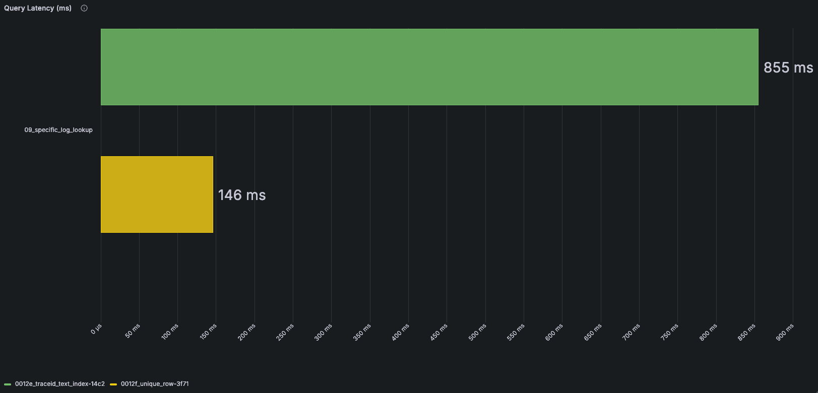
 The green bars here represent bloom filters; the yellow bars represent full-text search. Queries using a full-text search index have a higher floor due to index evaluation, but scale well with increased volume. The increase in evaluation is evident in the specific log lookup query — the upcoming block offset optimization mitigates this regression.
The 09_specific_log_lookup query is now degraded due to larger index evaluation of the text index compared to the bloom filter. The regression demonstrates how tricky schema changes are and why representative queries are so important for optimizing. This appears as a regression now, but will be addressed by the block offset and block number optimization mentioned later.
Furthermore, if the text index determines that a term exists in a row, ClickHouse can often satisfy part of the query directly from the index through the direct_read optimization. For highly selective searches, this avoids reading and decompressing large portions of the underlying column data, reducing both I/O and CPU overhead. This differs from the Bloom filter-based approach, which can only indicate that a granule might contain a match and still requires the data to be read and verified. As a result, text indexes are particularly effective for "needle-in-a-haystack" searches, where only a small fraction of rows contain the requested term, or any search filters on the Body that also request an aggregation e.g., count for the search histogram page.
TraceId as text index
As mentioned earlier, Bloom filters have an associated false positive rate. Text indexes do not, which makes them especially effective for highly selective searches. A TraceId lookup is a good example: the query is usually looking for one exact identifier across a very large volume of data. We thus decided to evaluate removing the Bloom filter from the TraceId column and using a text index instead.
-- Before
INDEX idx_trace_id TraceId TYPE bloom_filter(0.001) GRANULARITY 1,
-- After
INDEX idx_trace_id TraceId TYPE text(tokenizer='array'),As shown in the benchmark results below, replacing the Bloom filter with a text index improved TraceId searches by up to 22% in benchmarking, and scales well with increased volume.
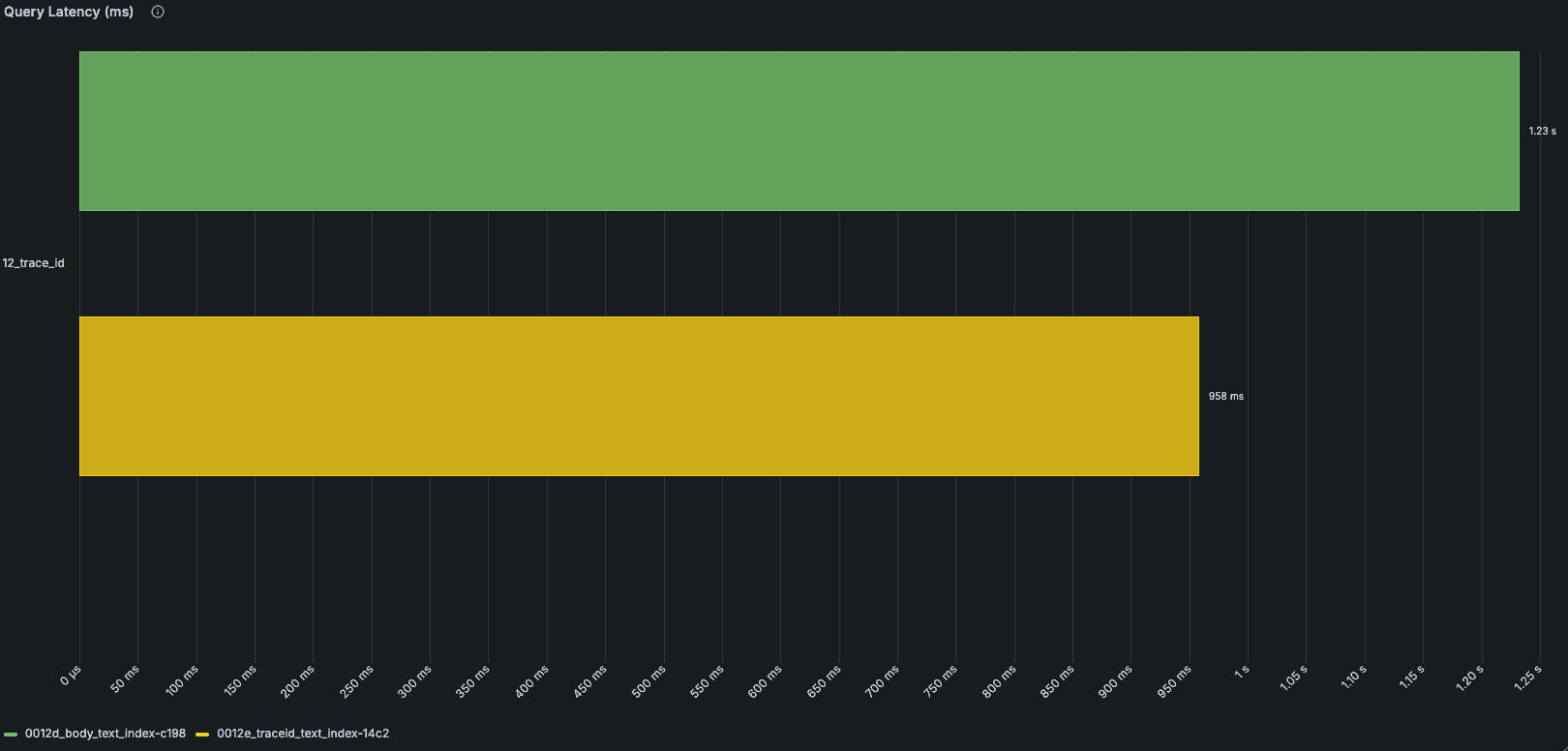
This does increase index storage, but because indexes reside in object storage, the additional cost is typically outweighed by the resulting improvements in query performance.
Block offset and block number settings
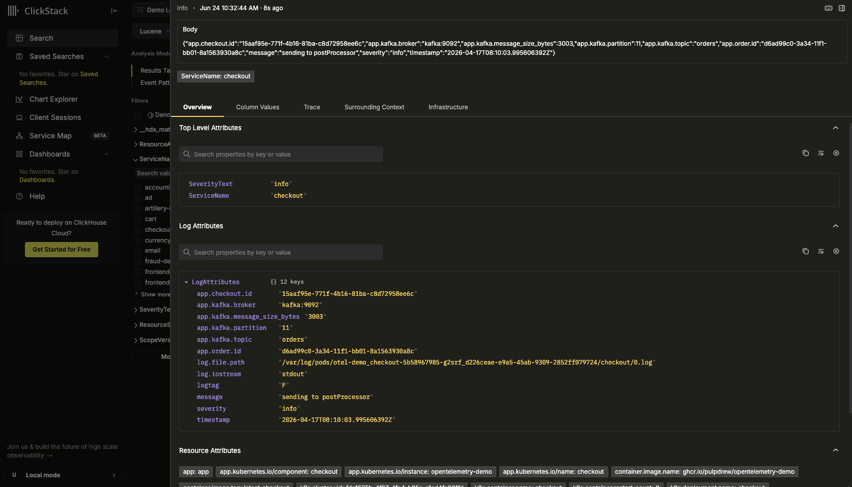
Many workflows in ClickStack ultimately require loading a single row. Viewing an individual log line is a common example. Search results typically return only a subset of columns to minimize data transfer and query cost, so when a user drills into a result, we need to fetch the complete row and all of its associated column values.
Identifying that row efficiently is not as straightforward as it might seem. ClickHouse's primary key is designed for data locality and pruning rather than uniqueness, meaning there may be multiple rows that share the same values for the columns returned by the initial search. Historically, ClickStack would use all returned column values as predicates when reloading the row. For example, if a search returned Timestamp, ServiceName, SeverityText, and Body, those values would all be included in the subsequent lookup query. This works, but requires filtering on additional columns and can result in more data being read than necessary.
The performance of this query also regressed after introducing text indexes due to their evaluation overhead. This motivated us to eliminate that overhead where possible.
ClickHouse provides a better mechanism through the _block_number and _block_offset virtual columns. Every inserted row belongs to a block, identified by _block_number, and has a unique position within that block, identified by _block_offset.
-- Before
SETTINGS index_granularity = 8192, ttl_only_drop_parts = 1;
-- After
SETTINGS index_granularity = 8192, ttl_only_drop_parts = 1, enable_block_number_column = 1, enable_block_offset_column = 1;By enabling the table settings required to persist these values, ClickStack can return them alongside search results and use them when fetching the full row.
This significantly simplifies the lookup query. Instead of filtering on many potentially large columns, ClickStack only needs the primary key columns together with _block_number and _block_offset to uniquely identify the row. Since the lookup is driven primarily by the primary key and a precise row location, fewer rows are examined, and the full record is retrieved more efficiently.
Materialized Views for better column autocomplete
Last year, we introduced materialized view support in ClickStack. Users could create materialized views tailored to their workload, register them with a source, and ClickStack would automatically use them whenever a query could be satisfied by the view instead of the underlying telemetry tables. This allowed users to shift work from query time to insert time, often resulting in substantial performance improvements.
As we gained more experience with the feature, we began looking for opportunities to apply the same approach elsewhere in the product. One area stood out immediately: autocomplete and filter value suggestions. Features such as the search sidebar and query builder rely on introspection of the underlying telemetry data to discover available attribute keys and values. Historically, this required querying the live otel_logs and otel_traces tables directly. While simple, the approach scaled poorly as datasets grew. Users were often forced to choose between slow introspection queries or sampled results that failed to surface enough values to be useful.
To address this, we started shipping materialized views as part of the default ClickStack schema. Rather than scanning telemetry tables at query time, ClickStack now maintains compact rollup tables dedicated to metadata discovery. These views use the AggregatingMergeTree engine to pre-aggregate (at insert time) attribute keys, values, and their frequencies in fifteen-minute buckets.
CREATE MATERIALIZED VIEW IF NOT EXISTS otel_logs_attr_kv_rollup_15m_mv
TO otel_logs_kv_rollup_15m
AS WITH elements AS (
SELECT 'NativeColumn' AS ColumnIdentifier,
toStartOfFifteenMinutes(Timestamp) AS Timestamp,
'SeverityText' AS Key,
CAST(SeverityText AS String) AS Value
FROM otel_logs
UNION ALL
-- similar UNION ALL branches for ServiceName, ScopeName, etc.
)
SELECT Timestamp, ColumnIdentifier, Key, Value, count() AS count
FROM elements
GROUP BY Timestamp, ColumnIdentifier, Key, Value;During source discovery, ClickStack automatically detects these rollups and routes autocomplete requests to them whenever available.
 Rollup tables are configured at a source level.
As a result, autocomplete queries no longer compete with normal search workloads. Suggestions can be fetched from a much smaller pre-aggregated dataset, significantly reducing latency on larger deployments. Because frequencies are tracked as part of the rollup process, results can also be ranked by popularity, producing more relevant suggestions without requiring an additional cache layer. What began as a user-configurable optimization has now become a core part of the default ClickStack experience.
Alias columns for maps to enable direct_read
This is a blog post where the best happens to be saved for last.
One of the most common and valid complaints about observability schemas is that accessing dynamic attributes can be slow. OpenTelemetry encourages enriching telemetry with arbitrary metadata, making it impossible to predict in advance every attribute a user may want to query. For this reason, ClickStack stores resource attributes, scope attributes, and log attributes using ClickHouse's Map type. This provides the flexibility required for observability workloads, but comes with a trade-off: querying a single key requires reading and parsing the entire map.
We've evaluated alternatives. The JSON type is particularly interesting because it can automatically materialize frequently accessed paths into dedicated subcolumns, reducing the amount of data that must be read at query time. In practice, however, the additional insert overhead is rarely justified for observability workloads where attributes are often sparse, highly variable, and continuously evolving. For now, maps remain the most practical representation for dynamic telemetry attributes.
More recently, sharded maps have emerged as another promising approach for reducing the cost of accessing individual map values. This feature complements the optimization below, which focuses on accelerating searches over map attributes rather than reducing the cost of reading them.
The original schema shown earlier already used Bloom filters on both map keys and map values. This could be used when evaluating conditions on a map.
INDEX idx_res_attr_key mapKeys(ResourceAttributes) TYPE bloom_filter(0.01) GRANULARITY 1,
INDEX idx_res_attr_value mapValues(ResourceAttributes) TYPE bloom_filter(0.01) GRANULARITY 1For example, when searching LogAttributes['foo'] = 'bar', one Bloom filter could eliminate granules where the key foo was absent, while another could eliminate granules where the value bar was absent. While this worked reasonably well, Bloom filters are probabilistic and operate at the granule level. Even after pruning, ClickHouse still needs to read and verify the remaining data, and false positives mean some granules may be read unnecessarily.
The success of text indexes on log bodies led us to ask whether we could apply the same approach to maps. Unlike Bloom filters, text indexes are exact and can participate in the direct_read optimization, allowing ClickHouse to satisfy highly selective searches directly from the index — without ever having to read the columns.
The challenge is that separate text indexes on map keys and map values can tell us that foo and bar exist in a row, but not whether they belong to the same key-value pair.
We accomplish this by concatenating each key with its value into a single string and storing that as an Array. The semantics look a bit funky, so we'll break it down.
ResourceAttributeItems Array(String) ALIAS arrayMap((arr) -> concat(arr.1, '=', arr.2), ResourceAttributes::Array(Tuple(String, String)))An ALIAS column is used so as not to store any of the data at rest. We only really want an index on this, and not the actual array value. The arrayMap function applies the provided lambda to each element of our ResourceAttributes map, which is internally represented as an array of tuples. In the lambda, the key and value are concatenated with a = separator.
At query time, we transform equality queries into an operation on the text index. For example, ResourceAttributes['foo']='bar' becomes has(ResourceAttributeItems, concat('foo', '=', 'bar')). This allows us to use the text index and, most importantly, the direct_read optimization. The pain of loading maps at query time is effectively gone for any strict equality operations. All queries benefit greatly from this, with some seeing up to 10x improvements in benchmarks.
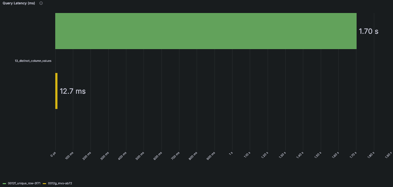
 The green bars represent Bloom filters, while the yellow bars show text indexes using the direct_read optimization.
An added bonus is that text indexes are themselves searchable. Because the index is organized by token, it can efficiently support prefix lookups using startsWith. This opens up new possibilities for introspection. For example, by indexing concatenated key-value pairs, we can quickly discover distinct values for a given key by querying for tokens that begin with foo=. ClickStack uses these capabilities to power autocomplete, filter suggestions, and other metadata-driven features throughout the application, all without scanning the underlying telemetry data. The key and value introspection query improvements open up entire product features that were previously impractical.
 The green bars represent the previous ClickStack introspection queries, while the yellow bars show introspection powered by these same text indices.
Conclusion
The optimizations described above have all been incorporated into the default ClickStack schema. Together, they address the most common observability query patterns while balancing query performance, ingestion efficiency, storage overhead, and operational complexity. The resulting schema looks substantially different from the one we started with, reflecting months of benchmarking, iteration, and validation against real-world workloads.
CREATE TABLE IF NOT EXISTS ${DATABASE}.otel_logs (
`Timestamp` DateTime64(9) CODEC(Delta(8), ZSTD(1)),
`TraceId` String CODEC(ZSTD(1)),
`SpanId` String CODEC(ZSTD(1)),
`TraceFlags` UInt8,
`SeverityText` LowCardinality(String) CODEC(ZSTD(1)),
`SeverityNumber` UInt8,
`ServiceName` LowCardinality(String) CODEC(ZSTD(1)),
`Body` String CODEC(ZSTD(1)),
`ResourceSchemaUrl` LowCardinality(String) CODEC(ZSTD(1)),
`ResourceAttributes` Map(LowCardinality(String), String) CODEC(ZSTD(1)),
`ScopeSchemaUrl` LowCardinality(String) CODEC(ZSTD(1)),
`ScopeName` String CODEC(ZSTD(1)),
`ScopeVersion` LowCardinality(String) CODEC(ZSTD(1)),
`ScopeAttributes` Map(LowCardinality(String), String) CODEC(ZSTD(1)),
`LogAttributes` Map(LowCardinality(String), String) CODEC(ZSTD(1)),
`EventName` String CODEC(ZSTD(1)),
`__hdx_materialized_k8s.cluster.name` LowCardinality(String) MATERIALIZED ResourceAttributes['k8s.cluster.name'] CODEC(ZSTD(1)),
`__hdx_materialized_k8s.container.name` LowCardinality(String) MATERIALIZED ResourceAttributes['k8s.container.name'] CODEC(ZSTD(1)),
`__hdx_materialized_k8s.deployment.name` LowCardinality(String) MATERIALIZED ResourceAttributes['k8s.deployment.name'] CODEC(ZSTD(1)),
`__hdx_materialized_k8s.namespace.name` LowCardinality(String) MATERIALIZED ResourceAttributes['k8s.namespace.name'] CODEC(ZSTD(1)),
`__hdx_materialized_k8s.node.name` LowCardinality(String) MATERIALIZED ResourceAttributes['k8s.node.name'] CODEC(ZSTD(1)),
`__hdx_materialized_k8s.pod.name` LowCardinality(String) MATERIALIZED ResourceAttributes['k8s.pod.name'] CODEC(ZSTD(1)),
`__hdx_materialized_k8s.pod.uid` LowCardinality(String) MATERIALIZED ResourceAttributes['k8s.pod.uid'] CODEC(ZSTD(1)),
`__hdx_materialized_deployment.environment.name` LowCardinality(String) MATERIALIZED ResourceAttributes['deployment.environment.name'] CODEC(ZSTD(1)),
`ResourceAttributeItems` Array(String) ALIAS arrayMap((arr) -> concat(arr.1, '=', arr.2), ResourceAttributes::Array(Tuple(String, String))),
`ScopeAttributeItems` Array(String) ALIAS arrayMap((arr) -> concat(arr.1, '=', arr.2), ScopeAttributes::Array(Tuple(String, String))),
`LogAttributeItems` Array(String) ALIAS arrayMap((arr) -> concat(arr.1, '=', arr.2), LogAttributes::Array(Tuple(String, String))),
INDEX idx_trace_id TraceId TYPE text(tokenizer = 'array'),
INDEX idx_res_attr_key mapKeys(ResourceAttributes) TYPE text(tokenizer = 'array'),
INDEX idx_res_attr_items ResourceAttributeItems TYPE text(tokenizer = 'array'),
INDEX idx_scope_attr_key mapKeys(ScopeAttributes) TYPE text(tokenizer = 'array'),
INDEX idx_scope_attr_items ScopeAttributeItems TYPE text(tokenizer = 'array'),
INDEX idx_log_attr_key mapKeys(LogAttributes) TYPE text(tokenizer = 'array'),
INDEX idx_log_attr_items LogAttributeItems TYPE text(tokenizer = 'array'),
INDEX idx_lower_body lower(Body) TYPE text(tokenizer = 'splitByNonAlpha')
)
ENGINE = MergeTree
PARTITION BY toDate(Timestamp)
ORDER BY (toStartOfFiveMinutes(Timestamp), ServiceName, Timestamp)
TTL toDateTime(Timestamp) + ${TABLES_TTL}
SETTINGS index_granularity = 8192, ttl_only_drop_parts = 1, enable_block_number_column = 1, enable_block_offset_column = 1;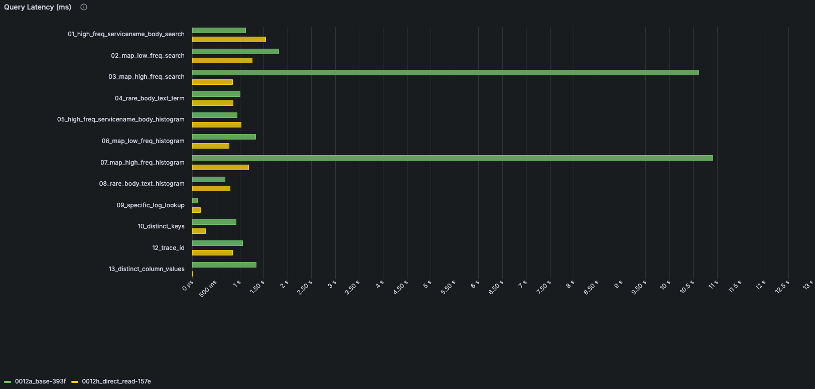
 Green bars represent the previous schema, while yellow bars represent the optimized schema. Query 11 is shown separately because of its larger scale.
The results have already paid dividends. Queries that previously struggled at scale now benefit from improvements across multiple layers of the stack, from primary key design and text indexes to alias columns and materialized views. Rather than relying on isolated optimizations for specific workloads, the schemas now provide a strong general-purpose foundation. Just as importantly, many of the techniques described here build on native ClickHouse features, allowing us to benefit from ongoing improvements in the database itself as new releases become available.
This work is only one part of the story. In the next post in this series, we'll explore how we used ClickCannon and this evolved schema to build a comprehensive benchmarking framework for ClickStack. We'll look at how we modeled observability workloads, how we translated throughput into infrastructure requirements, and what the resulting benchmarks tell us about the cost of operating ClickStack at scale.
Get started today
Interested in seeing how ClickHouse works on your data? Get started with ClickHouse Cloud in minutes and receive $300 in free credits.
Sign up