50k
50k
In financial services, market data systems typically split into two tiers: real-time and historical.
The real-time tier handles the live feed and the current trading day, serving queries that need answers in microseconds. And then, there's the historical tier, a durable archive of every prior day, that serves queries for research, backtesting, transaction-cost analysis, and regulatory reconstruction.
The historical tier is also the lowest-risk place to try a new database - it doesn't touch the live trading path, doesn't need microsecond latency, and the workload is well-understood (which makes it easy to test).
In this post, we load real tick data from Binance's public archive and show that ClickHouse stores it cheaply, queries it quickly, and handles the operations that matter to a trading desk: VWAP, OHLC candles, and as-of joins.
Why ClickHouse for historical ticker data?
Before the worked example, a brief word on why ClickHouse is well-suited to this workload. It comes down to two things: how it stores data, and how you query it.
Cost-efficiency
Unlike row-oriented databases, which store each record separately, ClickHouse stores data as columns, with values stored together on disk. For analytical workloads, this has a significant consequence for storage efficiency.
Storing similar data next to each other allows us to apply compression techniques to reduce the space they occupy. For example:
- Dictionary encoding saves space when a column has low cardinality. Instead of storing the same string thousands of times, we store a dictionary of distinct values and an integer reference per row.
- Delta encoding works well for timestamps or any column where adjacent values are monotonically increasing and differ by small amounts. Rather than storing the full value each time, we store only the difference from the previous value.
- Run-length encoding replaces a sequence of identical adjacent values with a single value and a count.
Tick data tends to compress particularly well because it has exactly these properties: timestamps that increment in small regular steps, prices that drift slowly, symbols that repeat millions of times, and trade IDs that increase monotonically.
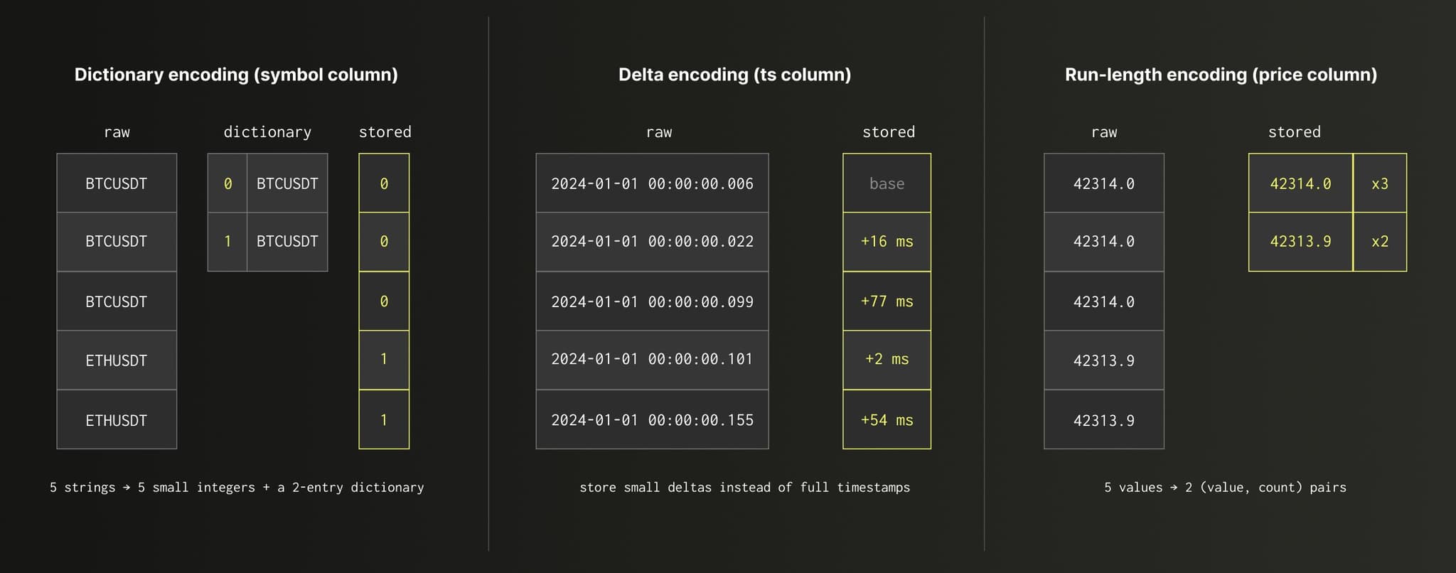
Beyond these specialized encodings, storing similar values together creates highly repetitive byte patterns that general-purpose compression algorithms such as ZSTD and LZ4 can exploit. These are applied to every column to reduce the amount of data stored.
Query accessibility
The second reason to consider ClickHouse for historical tick data is its ease of querying. ClickHouse uses SQL - the common language across data engineering, analytics, and business intelligence. According to the 2025 Stack Overflow Developer survey, 58.6% of developers use it.
There's no specialist language to learn, no small talent pool to hire from, and no bottleneck of having to route every question through the people who can write the queries. We'll see this in action in the worked examples below.
A worked example: Using ClickHouse for historical ticker data
Now we're going to have a look at a worked example showing how to use ClickHouse to query historical ticker data. We'll use Binance's public market-data archive, a free, openly redistributable dataset containing billions of records.
One month of data on clickhouse-local
We'll start with an example that you can run on your own computer - one month of USD-M perpetual futures (from January 2024) across five of the most active symbols - BTC, ETH, SOL, BNB, and XRP.
That gives us hundreds of millions of trades and nearly 2 billion quotes. You can use this script to download the data, which consists of 155 ZIP files totaling 21 GB.
Trades
Let's start with trades. A trade is a single executed transaction - the moment a buyer and seller agree on a price and quantity changed hands.
Each trade has a symbol, a timestamp (down to the millisecond), and the price and quantity that changed hands. We also have the notional value of the trade, quote_qty (price × quantity, in USDT), a unique, monotonically increasing trade ID, and a flag, is_buyer_maker, indicating which side was the aggressor.
CREATE TABLE trades
(
symbol LowCardinality(String),
ts DateTime64(3) CODEC(DoubleDelta, ZSTD(1)),
price Decimal(12, 2) CODEC(ZSTD(1)),
qty Decimal(16, 6) CODEC(ZSTD(1)),
quote_qty Decimal(20, 6) CODEC(ZSTD(1)),
trade_id UInt64 CODEC(DoubleDelta, ZSTD(1)),
is_buyer_maker Boolean CODEC(ZSTD(1))
)
ENGINE = MergeTree
ORDER BY (symbol, ts);Next, let's ingest the trades into our table:
INSERT INTO trades SELECT
splitByChar('-', _file)[1] AS symbol,
fromUnixTimestamp64Milli(time),
price, qty, quote_qty, id, is_buyer_maker
FROM file('data/*-trades-*.zip :: *.csv', CSVWithNames);You'll notice that we can query the archive files directly, a feature that's been in ClickHouse since version 23.8. It takes a little under 90 seconds to ingest this data:
373502424 rows in set. Elapsed: 81.706 sec. Processed 373.50 million rows, 19.38 GB (4.57 million rows/s., 237.17 MB/s.)
Peak memory usage: 226.02 MiB.Now that we've got the trades data loaded, let's compute the Volume-Weighted Average Price (VWAP) across all symbols for a single day.
VWAP is the average price at which an asset traded, weighted by the volume traded at each price level. It's one of the most-used benchmarks on a trading desk: funds measure execution quality against it, algorithms try to track it, and it's the standard answer to "what was the fair price for this asset today?"
It's computed by summing the notional value of every trade (quote_qty, which is price × qty) and dividing it by the total quantity traded. In the following query, we order symbols by notional volume traded (the amount of money that changed hands) rather than the number of units:
WITH
sum(quote_qty) AS raw_volume_usdt,
sum(qty) AS raw_volume_base
SELECT
symbol,
round(sum(quote_qty) / sum(qty), 2) AS vwap,
formatReadableQuantity(raw_volume_base) AS volume_base,
formatReadableQuantity(raw_volume_usdt) AS volume_usdt,
bar(raw_volume_usdt, 0, 13440000000, 20) AS chart
FROM trades
WHERE toDate(ts) = '2024-01-31'
GROUP BY symbol
ORDER BY raw_volume_usdt DESC;┌─symbol──┬─────vwap─┬─volume_base─────┬─volume_usdt────┬─chart────────────────┐
│ BTCUSDT │ 42940.53 │ 313.07 thousand │ 13.44 billion │ ████████████████████ │
│ ETHUSDT │ 2314.4 │ 2.61 million │ 6.04 billion │ ████████▉ │
│ SOLUSDT │ 99.82 │ 36.56 million │ 3.65 billion │ █████▍ │
│ XRPUSDT │ 0.5 │ 1.47 billion │ 740.63 million │ █ │
│ BNBUSDT │ 303.86 │ 883.20 thousand │ 268.37 million │ ▍ │
└─────────┴──────────┴─────────────────┴────────────────┴──────────────────────┘
5 rows in set. Elapsed: 0.126 sec. Processed 12.36 million rows, 308.92 MB (97.74 million rows/s., 2.44 GB/s.)
Peak memory usage: 621.91 KiB.In terms of volume, XRP has the most activity, but each one is worth only $0.50, putting it fourth in terms of money traded. BTC's $13.4 billion dwarfs the rest despite having the fewest units.
Next, let's write a query for an OHLC (Open, High, Low, Close) candle for a given symbol on a given day. The following query computes this for Bitcoin for each hour on the 16th January 2024:
SELECT toStartOfInterval(ts, INTERVAL 1 HOUR)::Time AS bucket,
argMin(price, ts) AS open,
max(price) AS high,
min(price) AS low,
argMax(price, ts) AS close,
round(sum(qty), 2) AS volume
FROM trades
WHERE symbol = 'BTCUSDT' AND toDate(ts) = '2024-01-16'
GROUP BY bucket
ORDER BY bucket;┌───bucket─┬────open─┬────high─┬─────low─┬───close─┬───volume─┐
│ 00:00:00 │ 42515 │ 42679 │ 42466.1 │ 42604.7 │ 4807.99 │
│ 01:00:00 │ 42604.6 │ 42733.7 │ 42556.6 │ 42591.7 │ 4728.84 │
│ 02:00:00 │ 42591.7 │ 42732.8 │ 42552 │ 42702.1 │ 5519.02 │
│ 03:00:00 │ 42702.1 │ 42942 │ 42695.7 │ 42921.2 │ 7032.13 │
│ 04:00:00 │ 42919.3 │ 42945 │ 42759.9 │ 42805.2 │ 5516.79 │
│ 05:00:00 │ 42805.2 │ 42932.5 │ 42759 │ 42765.3 │ 4148.77 │
│ 06:00:00 │ 42765.4 │ 42779.1 │ 42648.3 │ 42744.4 │ 5399.94 │
│ 07:00:00 │ 42744.5 │ 42788.1 │ 42600.5 │ 42788 │ 4965.14 │
│ 08:00:00 │ 42788.5 │ 43029.7 │ 42718.8 │ 43021.5 │ 8975.58 │
│ 09:00:00 │ 43021.5 │ 43164.9 │ 42899.6 │ 42937 │ 12361.57 │
│ 10:00:00 │ 42937.1 │ 42969.1 │ 42850.1 │ 42870 │ 4996.4 │
│ 11:00:00 │ 42870 │ 42944 │ 42753.6 │ 42895.3 │ 5799.53 │
│ 12:00:00 │ 42894.6 │ 43170 │ 42854.7 │ 43160.1 │ 10657.02 │
│ 13:00:00 │ 43160.1 │ 43181.7 │ 42705.6 │ 42805.7 │ 13452.14 │
│ 14:00:00 │ 42805.6 │ 42954.9 │ 42050 │ 42700.1 │ 55063.01 │
│ 15:00:00 │ 42700.1 │ 43333 │ 42545.6 │ 43251.7 │ 42560.65 │
│ 16:00:00 │ 43250.6 │ 43450 │ 43003.2 │ 43249.8 │ 24381.08 │
│ 17:00:00 │ 43249.8 │ 43249.8 │ 43027.6 │ 43046.6 │ 8896.75 │
│ 18:00:00 │ 43051.4 │ 43159.9 │ 42825.5 │ 43008.8 │ 10532.47 │
│ 19:00:00 │ 43008.8 │ 43182.3 │ 42940.8 │ 43164.8 │ 6539.24 │
│ 20:00:00 │ 43164.8 │ 43376.2 │ 43061.7 │ 43195.9 │ 13191 │
│ 21:00:00 │ 43195.9 │ 43589 │ 43181.6 │ 43427.5 │ 14845.85 │
│ 22:00:00 │ 43427.4 │ 43499.2 │ 43200 │ 43208.6 │ 6772.76 │
│ 23:00:00 │ 43208.6 │ 43285 │ 43105.2 │ 43133 │ 6063.55 │
└──────────┴─────────┴─────────┴─────────┴─────────┴──────────┘
24 rows in set. Elapsed: 0.041 sec. Processed 3.62 million rows, 90.24 MB (87.39 million rows/s., 2.18 GB/s.)
Peak memory usage: 5.28 MiB.Below is a chart generated using plot.ly that visualizes the data:
The price drifted up throughout the day, opening at $42,515 and closing at $43,133, a 1.5% intraday gain.
The 14:00 hour is the most interesting. During that hour, the price briefly crashed to $42,050 ( about $750 below where it started) before recovering. Trading activity was also unusually heavy: 55,063 BTC changed hands, more than 5x the typical hourly volume.
A wave of sellers drove the price down sharply, but enough buyers stepped in to push it back up within the same hour. What we can't see is when, within that hour, the selling was most intense.
That's what we'll look at next. The following query finds the one-minute interval where the price was at its lowest point between 14:00 and 15:00
SELECT
toStartOfMinute(ts) AS minute, count() AS trades,
round(min(price), 2) AS low, round(max(price), 2) AS high,
round(sum(qty), 3) AS volume
FROM trades
WHERE symbol = 'BTCUSDT'
AND ts >= '2024-01-16 14:00:00'
AND ts < '2024-01-16 15:00:00'
GROUP BY minute
ORDER BY low ASC
LIMIT 10;┌──────────────minute─┬─trades─┬─────low─┬────high─┬───volume─┐
│ 2024-01-16 14:44:00 │ 17191 │ 42050 │ 42167 │ 2494.94 │
│ 2024-01-16 14:45:00 │ 16390 │ 42090.2 │ 42212.8 │ 2053.689 │
│ 2024-01-16 14:43:00 │ 15723 │ 42115 │ 42244.4 │ 1914.875 │
│ 2024-01-16 14:46:00 │ 16682 │ 42143.2 │ 42275.2 │ 2163.598 │
│ 2024-01-16 14:42:00 │ 18611 │ 42152 │ 42273.4 │ 2241.841 │
│ 2024-01-16 14:47:00 │ 9863 │ 42175 │ 42278.6 │ 1106.466 │
│ 2024-01-16 14:48:00 │ 6575 │ 42187.3 │ 42265.3 │ 793.072 │
│ 2024-01-16 14:41:00 │ 10948 │ 42243.2 │ 42341.2 │ 1268.806 │
│ 2024-01-16 14:40:00 │ 15944 │ 42247.5 │ 42389.5 │ 1858.954 │
│ 2024-01-16 14:49:00 │ 9880 │ 42256.9 │ 42321.9 │ 1225.524 │
└─────────────────────┴────────┴─────────┴─────────┴──────────┘
10 rows in set. Elapsed: 0.017 sec. Processed 524.29 thousand rows, 12.69 MB (30.45 million rows/s., 736.98 MB/s.)
Peak memory usage: 62.55 KiB.The sell-off wasn't over in a single moment - the five minutes from 14:42 to 14:46 all show heavy trading activity and big price swings, as selling intensified and then gradually eased. But 14:44 looks like the worst of it. The price hit its lowest point of the entire hour ($42,050), and 2,494 BTC changed hands in sixty seconds.
But knowing when it happened only gets us so far. The hourly view can't tell us how it happened: was the price dropping because there were barely any buyers around, meaning each sale pushed it down further? Or were there genuinely buyers and sellers active on both sides, holding the price steady even under pressure?
To answer that, we need to look at each trade individually, alongside the market price at the time it was executed.
Quotes
While the trades table recorded what actually happened, the quotes table records what could have happened at each instant. Each record captures the best bid (the highest price a buyer was willing to pay) and the best ask (the lowest price a seller was willing to accept) at every moment the order book changed.
Our table will also include bid_qty, the amount someone wants to buy at the highest price, and ask_qty, the amount someone wants to sell at the lowest price. symbol and ts are self-explanatory! update_id is a monotonically increasing integer.
Every time the best bid or best ask changes (e.g., when an order is placed, canceled, or filled), Binance adds a new record to the quotes table.
The schema for the quotes table is shown below:
CREATE TABLE quotes
(
symbol LowCardinality(String),
ts DateTime64(3) CODEC(DoubleDelta, ZSTD(1)),
bid_price Decimal(12, 4) CODEC(ZSTD(1)),
bid_qty Decimal(16, 3) CODEC(ZSTD(1)),
ask_price Decimal(12, 4) CODEC(ZSTD(1)),
ask_qty Decimal(16, 3) CODEC(ZSTD(1)),
update_id UInt64 CODEC(DoubleDelta, ZSTD(1))
)
ENGINE = MergeTree
ORDER BY (symbol, ts);And we can ingest the data using the following query:
INSERT INTO quotes SELECT
splitByChar('-', _file)[1] AS symbol,
fromUnixTimestamp64Milli(transaction_time),
best_bid_price, best_bid_qty, best_ask_price, best_ask_qty, update_id
FROM file('data/*-bookTicker-*.zip :: *.csv', CSVWithNames);To ingest just under 2 billion records takes around 8 minutes:
1997061823 rows in set. Elapsed: 509.946 sec. Processed 2.00 billion rows, 185.91 GB (3.92 million rows/s., 364.57 MB/s.)
Peak memory usage: 273.32 MiB.Now that we've loaded the quotes, we can resume investigating the trade activity at 14:44 on 16th January 2024.
To analyze this activity, we'll use an ASOF JOIN - a join that matches each trade to the most recent quote available at the moment it happened. This tells us not just what price a trade executed at, but what price was being advertised in the market at that exact instant.
The query breaks that one-minute window into per-second snapshots, showing for each second: how many trades happened, the price range, total volume, and average slippage.
Slippage measures how far the actual trade price strayed from the advertised price - when a large wave of selling overwhelms the available buyers, trades start executing at worse and worse prices, and slippage spikes. Once the selling eases and buyers return, it drops back down.
SELECT
toStartOfSecond(t.ts) AS second, count() AS trades,
round(min(t.price), 2) AS low, round(max(t.price), 2) AS high,
round(sum(t.qty), 3) AS volume,
round(avg(abs(t.price - (q.bid_price + q.ask_price) / 2)), 4) AS avg_slippage
FROM (
SELECT ts, price, qty, symbol
FROM trades
WHERE symbol = 'BTCUSDT'
AND ts >= '2024-01-16 14:44:00' AND ts < '2024-01-16 14:45:00'
) AS t
ASOF JOIN (
SELECT ts, bid_price, ask_price, symbol
FROM quotes
WHERE symbol = 'BTCUSDT'
AND ts >= '2024-01-16 14:44:00' AND ts < '2024-01-16 14:45:00'
) AS q
ON t.symbol = q.symbol AND t.ts >= q.ts
GROUP BY second
ORDER BY second;┌──────────────────second─┬─trades─┬─────low─┬────high─┬──volume─┬─avg_slippage─┐
│ 2024-01-16 14:44:00.000 │ 172 │ 42163.5 │ 42167 │ 94.074 │ 0.1831 │
│ 2024-01-16 14:44:01.000 │ 131 │ 42157.6 │ 42166.9 │ 16.363 │ 0.1912 │
│ 2024-01-16 14:44:02.000 │ 557 │ 42138.3 │ 42157.7 │ 44.769 │ 0.2707 │
│ 2024-01-16 14:44:03.000 │ 296 │ 42135 │ 42147.2 │ 37.372 │ 0.81 │
│ 2024-01-16 14:44:04.000 │ 190 │ 42135.5 │ 42149.7 │ 18.159 │ 0.3334 │
│ 2024-01-16 14:44:05.000 │ 221 │ 42139.5 │ 42166.8 │ 25.645 │ 0.6104 │
│ 2024-01-16 14:44:06.000 │ 136 │ 42155.5 │ 42166.8 │ 10.639 │ 0.1783 │
│ 2024-01-16 14:44:07.000 │ 90 │ 42147 │ 42155.5 │ 5.536 │ 0.2694 │
│ 2024-01-16 14:44:08.000 │ 259 │ 42136 │ 42150.4 │ 20.764 │ 0.873 │
│ 2024-01-16 14:44:09.000 │ 83 │ 42146.6 │ 42152.1 │ 10.873 │ 0.2054 │
│ 2024-01-16 14:44:10.000 │ 221 │ 42135 │ 42146.7 │ 32.567 │ 0.6351 │
│ 2024-01-16 14:44:11.000 │ 212 │ 42123.3 │ 42135.1 │ 15.032 │ 0.3255 │
│ 2024-01-16 14:44:12.000 │ 1162 │ 42106 │ 42138.8 │ 319.489 │ 3.973 │
│ 2024-01-16 14:44:13.000 │ 2529 │ 42055.2 │ 42116.2 │ 324.301 │ 1.8386 │
│ 2024-01-16 14:44:14.000 │ 1231 │ 42055.3 │ 42091.9 │ 170.522 │ 1.9567 │
│ 2024-01-16 14:44:15.000 │ 1990 │ 42050 │ 42116.5 │ 304.494 │ 13.0489 │
│ 2024-01-16 14:44:16.000 │ 511 │ 42071 │ 42092.1 │ 57.994 │ 1.3883 │
│ 2024-01-16 14:44:17.000 │ 370 │ 42070.5 │ 42101.1 │ 69.605 │ 3.0209 │
│ 2024-01-16 14:44:18.000 │ 240 │ 42094.2 │ 42108 │ 24.206 │ 1.13 │
│ 2024-01-16 14:44:19.000 │ 176 │ 42081.6 │ 42095 │ 19.469 │ 1.3463 │
│ 2024-01-16 14:44:20.000 │ 209 │ 42081.6 │ 42100 │ 19.652 │ 0.8911 │
│ 2024-01-16 14:44:21.000 │ 231 │ 42087.3 │ 42104.4 │ 26.879 │ 1.082 │
│ 2024-01-16 14:44:22.000 │ 90 │ 42087.3 │ 42088.8 │ 5.938 │ 0.0767 │
│ 2024-01-16 14:44:23.000 │ 235 │ 42089.5 │ 42100.1 │ 26.002 │ 1.7451 │
....
│ 2024-01-16 14:44:57.000 │ 453 │ 42095 │ 42114.4 │ 56.588 │ 2.7029 │
│ 2024-01-16 14:44:58.000 │ 169 │ 42100.4 │ 42110 │ 13.492 │ 0.6219 │
│ 2024-01-16 14:44:59.000 │ 151 │ 42101.8 │ 42107.4 │ 6.062 │ 1.2255 │
└──────────────────second─┴─trades─┴─────low─┴────high─┴──volume─┴─avg_slippage─┘
60 rows in set. Elapsed: 0.053 sec. Processed 155.65 thousand rows, 2.36 MB (2.93 million rows/s., 44.38 MB/s.)
Peak memory usage: 1.92 MiB.The results reveal three distinct phases within that single minute, which are easier to see on this visualization:
The build-up (00-11). The price is already falling from $42,167 at the open of the minute to $42,123 by second 11, but the market is still functioning normally. Trade counts are modest (83–557 per second), volume is low, and average slippage is $0.18–$0.87. Sellers are in control, but liquidity is holding.
The crash (12-15). In four seconds, everything changes. Trade counts explode - 1,162, then 2,529, then 1,231, then 1,990 trades per second. Volume spikes to 300+ BTC per second. Price collapses from $42,138 to $42,050. And at 15, average slippage hits $13.05 - 260× the half-tick baseline. The order book has been swept clean; buyers are paying whatever it takes to get filled.
The recovery (16 onwards). As quickly as it broke, the market stabilized. By 22, slippage is back to $0.08. By 30, trade counts are back to normal. The price settles around $42,095-42,105 and holds there for the rest of the minute. The whole event took 15 seconds.
We might want to then drill down into the other minutes to see if something similar was happening, but we'll leave that as an exercise for the reader!
Amount of space taken
But before you go exploring, it's worth knowing how much space all this data actually takes up.
The raw ZIP files for one month take up 21 GiB of space, but after unzipping, the total is 191 GiB. And we can run the following query to compute the amount of space taken by each of our tables in ClickHouse:
SELECT table,
formatReadableSize(sum(bytes_on_disk)) AS on_disk
FROM system.parts
WHERE active AND database = currentDatabase() AND table IN ('trades', 'quotes')
GROUP BY table;┌─table──┬─on_disk───┐
│ quotes │ 7.85 GiB │
│ trades │ 2.06 GiB │
└────────┴───────────┘One month of trade and quote data across five of the busiest futures pairs compresses to 10 GiB on disk, down from 191 GiB in raw CSV files, a 19x reduction.
Quotes compress better than trades because the bid and ask prices move slowly and predictably, which the codecs exploit well.
We can run the following query to compute a per-column breakdown for the trades table:
SELECT name,
formatReadableSize(sum(data_compressed_bytes)) AS on_disk,
round(sum(data_uncompressed_bytes)
/ sum(data_compressed_bytes), 1) AS ratio
FROM system.columns
WHERE database = currentDatabase()
AND table = 'trades'
GROUP BY name
ORDER BY sum(data_compressed_bytes) DESC;┌─name───────────┬─on_disk────┬─ratio─┐
│ quote_qty │ 1.11 GiB │ 5 │
│ qty │ 628.66 MiB │ 4.5 │
│ ts │ 175.32 MiB │ 16.2 │
│ price │ 115.87 MiB │ 24.6 │
│ is_buyer_maker │ 32.06 MiB │ 11.1 │
│ trade_id │ 9.75 MiB │ 292.1 │
│ symbol │ 1.70 MiB │ 209.9 │
└────────────────┴────────────┴───────┘ClickHouse's various codecs have done a good job of compressing the data.
There are only five unique values for symbol, which can be easily compressed by LowCardinality, which stores a dictionary of just those five values and replaces each row's string with an integer reference.
Timestamps are sorted and evenly spaced, and trade_id is a monotonically increasing counter, making them both ideal for DoubleDelta compression.
The two worst-compressed columns are qty and quote_qty, which are essentially random, so our codecs can't help much. quote_qty can be computed from qty and price, so if we wanted to reduce the space further, we might infer that column from the other two.
Almost one year of data on ClickHouse Cloud
Now we're going to scale this up to (almost) one year's worth of data, and instead of using my laptop, we'll use a ClickHouse Cloud service with 1 replica, 64 GiB of RAM, and 16 vCPUs.
We'll load data from May 2023 to March 2024. We would have liked to do a full year, but the quotes data stopped being published after March 2024.
10 months of ZIP files take up 162 GiB of space, or approximately 1.46 TB uncompressed, using a 9x multiplier that we saw when unzipping the local files.
We have a script that uses the Python client to load the data one day and one symbol at a time. It takes 886 seconds to load the trades and 1,972 seconds to load the quotes, running 16 insert statements in parallel.
Once the data's loaded, we can run the following query to see how much data we have and how much space it takes:
SELECT table, sum(rows) AS rows,
formatReadableSize(sum(bytes_on_disk)) AS on_disk
FROM system.parts
WHERE active AND table IN ('trades', 'quotes')
GROUP BY table;┌─table──┬────────rows─┬─on_disk───┐
│ quotes │ 13062612165 │ 58.20 GiB │
│ trades │ 3131315443 │ 18.61 GiB │
└────────┴─────────────┴───────────┘10 months of tick data for 5 of the busiest crypto futures pairs totals 16.2 billion rows and takes up 76 GiB of space, compressed. Again, that's about a 19x reduction from the space taken up by the raw CSV files.
ClickHouse Cloud storage is billed at $25.30 per 1 TB/mo, so our 10 months of tick data costs $3.29 per month.
$25.30 × (133 / 1024) = $25.30 × 0.07421875 = $1.88/month
The queries we ran locally all take roughly the same amount of time, even on a much larger dataset, because they can use the primary index to filter out irrelevant data.
Looking at the query plan of the first JOIN ASOF query helps see this:
┌─explain─────────────────────────────────────────────────────────────────────────────────────────────────────────────────────────────────────┐
│ Expression ((Project names + (Before ORDER BY + Projection) [lifted up part])) │
│ Sorting (Sorting for ORDER BY) │
│ Expression ((Before ORDER BY + Projection)) │
│ Aggregating │
│ Expression (Before GROUP BY) │
│ Expression (Post Join Actions) │
│ Join (JOIN FillRightFirst) │
│ Expression (Left Pre Join Actions) │
│ Expression ((Change column names to column identifiers + (Project names + Projection))) │
│ Expression ((WHERE + Change column names to column identifiers)) │
│ ReadFromMergeTree (default.trades) │
│ Indexes: │
│ PrimaryKey │
│ Keys: │
│ symbol │
│ ts │
│ Condition: and((ts in (-Inf, '1705416300')), and((ts in ['1705416240', +Inf)), (symbol in ['BTCUSDT', 'BTCUSDT']))) │
│ Parts: 2/3 │
│ Granules: 4/383083 │
│ Search Algorithm: binary search │
│ Ranges: 2 │
│ Expression (Right Pre Join Actions) │
│ Expression ((Change column names to column identifiers + (Project names + Projection))) │
│ Expression ((WHERE + Change column names to column identifiers)) │
│ ReadFromMergeTree (default.quotes) │
│ Indexes: │
│ PrimaryKey │
│ Keys: │
│ symbol │
│ ts │
│ Condition: and((ts in (-Inf, '1705416300')), and((ts in ['1705416240', +Inf)), (symbol in ['BTCUSDT', 'BTCUSDT']))) │
│ Parts: 9/9 │
│ Granules: 13/1597699 │
│ Search Algorithm: binary search │
│ Ranges: 9 │
└─────────────────────────────────────────────────────────────────────────────────────────────────────────────────────────────────────────────┘Lines 20 and 34 are the ones to look at. On line 20, the query engine reads only 4 of the 383,083 trades granules, and on line 34, it reads only 13 of 1,597,699 quotes granules.
There are 8,192 rows per granule, so we only need to read ~33,000 (0.001%) of the trades table and ~106,000 (0.0008%) of the quotes table.
The condition a couple of lines up explains how it knows which granules to read:
Condition: and((ts in (-Inf, '1705416300')), and((ts in ['1705416240', +Inf)), (symbol in ['BTCUSDT', 'BTCUSDT'])))
The primary key (symbol, ts) is sorted on disk. ClickHouse performs a binary search over the sparse index to find exactly which granules contain symbol = BTCUSDT and ts within the 60-second window, skipping everything else.
In summary
Hopefully, you now agree that ClickHouse handles historical tick data well!
Ten months of trades and quotes for five of the busiest futures pairs, or 16.2 billion rows, compressed to 76 GiB on disk, and costs $1.88 per month on ClickHouse Cloud. The codecs that make this possible are tuned to the structure of tick data: sorted timestamps, slowly drifting prices, and low-cardinality symbols.
And the analysis is just SQL. The operations a trading desk runs each day (VWAP, OHLC candles, and as-of joins) are all standard queries that any analyst can read, write, and extend.
Working with a 16-billion-row dataset doesn't change the latency for these queries. Since each query filters by symbol and time, the primary index skips a huge majority of the data before reading a single row.
Queries that don't filter on those dimensions will scan more, but for the typical tick-data workload - "this symbol, over this time range" - the index does exactly what you'd want.
Get started today
Interested in seeing how ClickHouse works on your data? Get started with ClickHouse Cloud in minutes and receive $300 in free credits.
Sign up