TL;DR
Over two years, ClickHouse became 26× faster on join-heavy analytical workloads. This post explains the engineering that made joins a first-class strength.
Two years of focused join engineering
ClickHouse is known for fast analytical queries, high compression, and real-time performance at scale.
Over the last two years, one major engineering focus has been bringing that same performance profile to join-heavy SQL queries.
At the ClickHouse 24.5 release webinar, Alexey Milovidov, inventor of ClickHouse, described the direction clearly:
“From now on, you will see JOIN improvements in every ClickHouse release.”
The chart below shows what that looked like in practice.

The first year laid the foundation: faster parallel hash join, smarter planning, aggressive filter pushdown, and local join reordering.
By 25.4, the same TPC-H SF100 join-heavy workload was already 4.4× faster than in 22.4.
The second year pushed much further. Between 25.4 and 26.4, a new wave of optimizer and execution improvements made the same workload another 6× faster with default settings.
End to end, ClickHouse is now 26× faster on TPC-H SF100 than it was in 22.4.
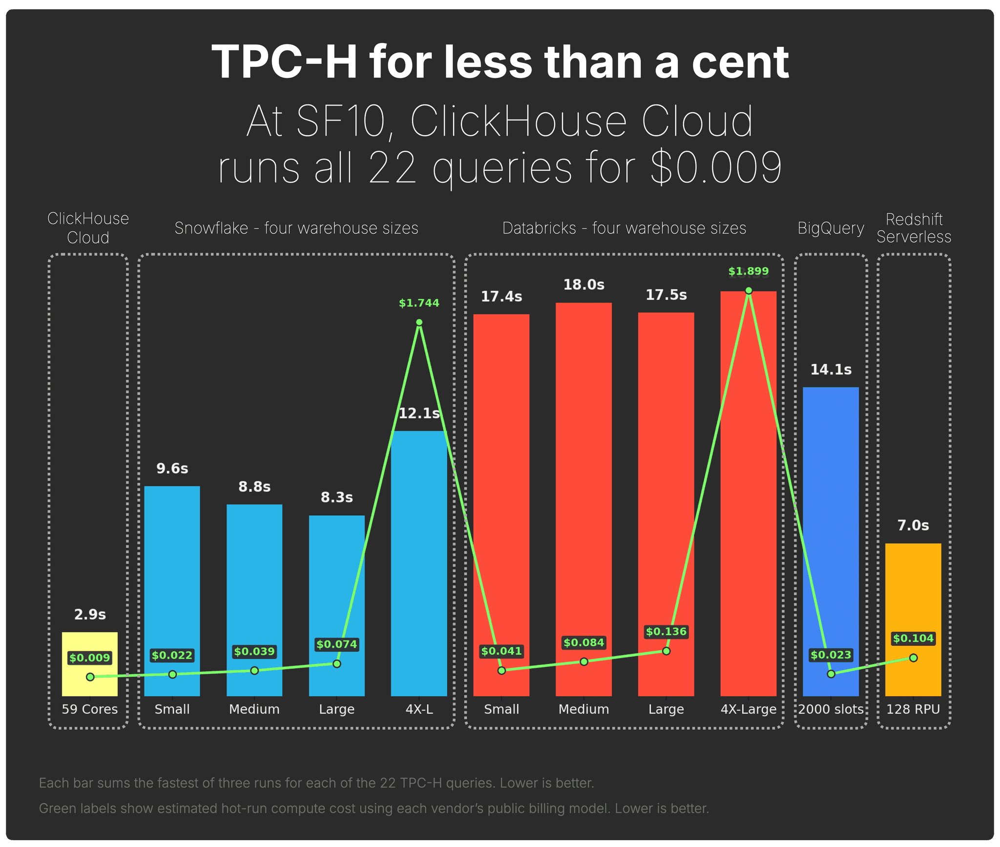
This post explains how we got there. The companion post shows what it unlocked: ClickHouse Cloud now runs TPC-H for less than a cent, and competes head-to-head with Snowflake, Databricks, BigQuery, and Redshift on SF100.
Year one: building the foundation
A year ago, at our first Open House user conference in San Francisco, ClickHouse join engineering lead, Robert Schulze, presented the first year of major join-performance work.
That first year was about building the foundation. ClickHouse made parallel hash join the default in 24.12, added local automatic join reordering for two-table joins, and delivered a steady stream of low-level execution improvements.
Several of those changes landed across consecutive releases:
- 24.7: improved hash table allocation for faster parallel hash joins
- 24.12: made parallel hash join the default strategy and introduced local automatic join reordering
- 25.1: sped up the hash join probe phase
- 25.2: removed thread contention in the hash join build phase
Together, those improvements made the same TPC-H SF100 join-heavy workload 4.4× faster by 25.4 compared with 22.4.
But year one was only the foundation. The second year is where joins became dramatically better with default settings.
Year two: making joins competitive by default
This year at Open House, Robert is back with the second chapter of the join-performance story.
Year one built the foundation. Year two made joins competitive with default settings.
The goal was simple: users should not have to rewrite queries, tune join orders by hand, or know which internal optimization to enable. ClickHouse should recognize more join-heavy SQL, automatically choose better plans, and avoid unnecessary work during execution.
The chart below shows the four main improvements that became effective by default between 25.4 and 26.4. Together, they made the same TPC-H SF100 join-heavy workload another 6× faster.

The rest of this post walks through those four improvements:
① Correlated subqueries in JOINs — support more real-world SQL directly.
② Lazy column replication — avoid copying repeated values produced by joins.
③ Runtime filters — skip probe-side rows before expensive hash-table lookups.
④ Statistics-based join reordering — choose better join plans automatically.
All examples use TPC-H SF100 on the same hardware, an AWS EC2 m6i.8xlarge instance (32 vCPUs, 128 GiB RAM), so the improvements are easy to compare.
① Correlated subqueries in JOINs
Two years ago, the problem was not just that some joins were slower than we wanted them to be. Some important join-heavy queries could not run at all.
Why this mattered
In the TPC-H benchmark section of our first research paper, presented at VLDB 2024, we had to exclude seven queries: Q2, Q4, Q13, Q17, and Q20–Q22. Because they used correlated subqueries, which ClickHouse did not fully support at the time.
A correlated TPC-H query
TPC-H Q4 is a good example. It contains an inner query over lineitem that references orders, the table from the outer query:

This is what makes it a correlated subquery: the inner query cannot be understood in isolation, because it depends on values from the outer query.
From row-by-row execution to set-oriented plans
Correlated subqueries are common because they are natural to write. They are also increasingly common in generated SQL, including queries produced by agentic systems. But for a database engine, they are hard to execute efficiently.
The naive plan is to evaluate the inner query once for every row from the outer query. That is simple, but often disastrous for performance. To make these queries fast, the optimizer has to decorrelate them: rewrite the query into an equivalent set-oriented plan, typically using joins, aggregations, semi joins, or anti joins.
That rewrite must preserve SQL semantics around duplicates, aggregates, and NULLs, which makes it much harder than it looks.
Result
Correlated subqueries are now first-class SQL in ClickHouse. Queries that previously required manual rewrites - including the excluded TPC-H queries - now run directly.
② Lazy column replication in JOINs
Lazy column replication reduces CPU and memory usage when JOINs logically repeat the same values many times.
The problem: logical repetition becomes physical copying
In JOIN results, one input row can produce many output rows. In TPC-H, for example, each customer can have multiple orders. When we join orders with customer, the customer columns are logically repeated once for every matching order.
SELECT
    o.o_orderkey,
    o.o_orderdate,
    c.c_name,
    c.c_address,
    c.c_comment
FROM orders AS o
INNER JOIN customer AS c
ON o.o_custkey = c.c_custkey;Logically, the result looks like this:

Conceptually, this is the correct result: the same customer values appear next to each matching order.
The expensive part is physical replication. If ClickHouse copies wide values such as c_address or c_comment into every joined row, the join spends CPU cycles and memory bandwidth duplicating the same data again and again. And if later operators like aggregations discard most of those rows, much of that copying was unnecessary.
Lazy column replication avoids that eager copying.
Instead of physically replicating repeated values during the join, ClickHouse keeps the original values once in a small dictionary data structure and represents the joined column as a compact index value pointing back to them:

If a later query step needs the fully materialized column, ClickHouse can still produce it. But many analytical operations can work directly on the compact representation, so the repeated values never need to be copied at all.
This is especially useful for JOINs that duplicate wide columns, such as strings.
Benchmark: avoiding physical replication
For the benchmark, we use a self-join on orders to create many repeated o_comment values, and then immediately consume them with cityHash64.
First, we ran the following example join without lazy replication.
SELECT sum(cityHash64(t1.o_comment))
FROM orders AS t1
INNER JOIN orders AS t2
    ON t1.o_custkey = t2.o_custkey
SETTINGS
    enable_lazy_columns_replication = 0,
allow_special_serialization_kinds_in_output_formats = 0;Fastest of three runs:
1 row in set. Elapsed: 5.419 sec. Processed 300.00 million rows, 8.89 GB (55.36 million rows/s., 1.64 GB/s.)
Peak memory usage: 5.27 GiB.Then, we ran the same query with lazy columns replication enabled.
This is the ideal case for lazy replication: o_comment is only needed as input to a function, so ClickHouse can evaluate cityHash64 over the compact representation without physically materializing the repeated string column.
SELECT sum(cityHash64(t1.o_comment))
FROM orders AS t1
INNER JOIN orders AS t2
    ON t1.o_custkey = t2.o_custkey
SETTINGS
    enable_lazy_columns_replication = 1,
allow_special_serialization_kinds_in_output_formats = 1;Fastest of three runs:
1 row in set. Elapsed: 2.847 sec. Processed 300.00 million rows, 8.89 GB (105.36 million rows/s., 3.12 GB/s.)
Peak memory usage: 5.22 GiB.Result
Result: Lazy column replication made this join 1.9× faster, reducing runtime from 5.419s to 2.847s, while slightly lowering peak memory usage from 5.27 GiB to 5.22 GiB.
The speedup comes from evaluating cityHash64 directly over the compact replicated-column representation rather than physically copying repeated strings.
③ Runtime filters in JOINs
Runtime filters reduce wasted probe-side work in hash joins.
They generalize a technique already used by ClickHouse’s full sorting merge join algorithm, where joined tables can be filtered by each other’s join keys before the join itself runs. ClickHouse introduces a similar idea for the default parallel hash join algorithm.
As a reminder, the parallel hash join algorithm is a variation of hash join that splits the input data to build several hash tables concurrently, speeding up the build phase.
In the example below, we set max_threads = 2, so ClickHouse builds two hash tables in parallel. In practice, max_threads is usually derived from the number of available CPU cores.
The diagram shows the physical query plan, called the query pipeline in ClickHouse, for a TPC-H query joining orders with customer.

① The predicate on customer is pushed down and applied before the join.
② During the build phase, the filtered customer rows, the right side of the join, are split into two buckets because max_threads = 2. Each bucket is used to build one in-memory hash table.
③ During the probe phase, orders rows, the left side of the join, are streamed in parallel and routed to the corresponding hash table for lookup.
The problem: wasted probe-side work
Note that in step ②, only a subset of customer keys is inserted into the hash tables during the build phase. However, in step ③, ClickHouse still processes all orders rows. For orders whose customer was removed by the customer filter, the lookup can never succeed. Those rows still consume CPU and memory bandwidth before the join rejects them.
The idea: filter probe rows before lookup
Runtime filters address exactly this wasted work.
While ClickHouse builds the hash tables (in DRAM) from the filtered customer rows, it also creates a compact filter (bloom filter or min/max values) from the join keys that actually made it into the build side. In our example, that means only customer keys that survived c_nation = 'DE'.
That filter is applied to the orders side before the hash-table lookup. If an orders row has an o_custkey that is not present in the filtered build side, ClickHouse can discard it early instead of routing it into the join.
The runtime filter is much smaller than the hash tables themselves, so it can stay close to the CPU, typically in L1 or L2 cache.
How runtime filters fit into the query pipeline
The updated pipeline looks like this:

The updated pipeline adds two steps:
② While reading the filtered customer rows, ClickHouse builds a runtime filter from their join keys.
④ Before probing the hash tables, ClickHouse applies that runtime filter to the orders rows.
⑤ Only rows that pass the runtime filter continue to the hash-table lookup.
The parallel hash join structure stays the same, but many probe-side rows are removed before the expensive lookup.
This keeps the parallel hash join structure unchanged, but removes probe-side rows that could never match. In selective joins, this can significantly reduce CPU work and memory bandwidth.
How it appears in the query plan
We can see this in the logical query plan with EXPLAIN plan.
First, with runtime pre-filtering disabled:
EXPLAIN plan
SELECT *
FROM orders, customer
WHERE o_custkey = c_custkey
SETTINGS enable_join_runtime_filters = 0;...
Join
...
ReadFromMergeTree (default.orders)
ReadFromMergeTree (default.customer)We’ll skip the rest of the plan and focus on the core mechanics.
Reading the output from bottom to top, we can see that ClickHouse plans to read the data from the two tables, orders and customer, and perform the join.
Next, let’s inspect the logical query plan for the same join, but this time with runtime pre-filtering enabled:
EXPLAIN plan
SELECT *
FROM orders, customer
WHERE o_custkey = c_custkey
SETTINGS enable_join_runtime_filters = 1;The relevant parts of the plan look like this:
...
Join
...
Prewhere filter column: __filterContains(_runtime_filter_14211390369232515712_0, __table1.o_custkey)
...
BuildRuntimeFilter (Build runtime join filter on __table2.c_custkey (_runtime_filter_14211390369232515712_0))
...Reading the plan from bottom to top, we can see that ClickHouse first ① builds a runtime filter from the join key values on the right-hand side (customer) table.
This runtime filter is then ② applied as a PREWHERE filter on the left-hand side (orders) table, allowing irrelevant rows to be skipped before the join is executed.
Benchmark: fewer rows, less memory
To measure the effect, we use a slightly extended version of the query, joining orders, customer, and nation, and calculating the average order total for customers from France.
We’ll start with runtime pre-filtering disabled:
SELECT avg(o_totalprice)
FROM orders, customer, nation
WHERE (c_custkey = o_custkey) AND (c_nationkey = n_nationkey) AND (n_name = 'FRANCE')
SETTINGS enable_join_runtime_filters = 0;┌──avg(o_totalprice)─┐
│ 151149.41468432106 │
└────────────────────┘
1 row in set. Elapsed: 1.005 sec. Processed 165.00 million rows, 1.92 GB (164.25 million rows/s., 1.91 GB/s.)
Peak memory usage: 1.24 GiB.Then, we run the same query again, this time with runtime pre-filtering enabled:
SELECT avg(o_totalprice)
FROM orders, customer, nation
WHERE (c_custkey = o_custkey) AND (c_nationkey = n_nationkey) AND (n_name = 'FRANCE')
SETTINGS enable_join_runtime_filters = 1;┌──avg(o_totalprice)─┐
│ 151149.41468432106 │
└────────────────────┘
1 row in set. Elapsed: 0.471 sec. Processed 165.00 million rows, 1.92 GB (350.64 million rows/s., 4.08 GB/s.)
Peak memory usage: 185.18 MiB.Result
Runtime pre-filtering made this query 2.1× faster, reducing runtime from 1.005s to 0.471s, while cutting peak memory from 1.24 GiB to 185 MiB.
By filtering rows early, ClickHouse avoids probe-side work that cannot produce matches, reducing both CPU work and memory usage.
④ Statistics-based join reordering
ClickHouse can now reorder complex join graphs across dozens of tables and all major join types.
This matters because SQL joins are associative: the same logical query can often be executed using many different join orders. The result is the same, but the runtime can be dramatically different.
The problem: join order matters
The diagram below shows three different join orders for the same join query and the resulting hash join trees. The query result will be the same in all three cases.

The more tables a query joins, the more important the join order becomes.
As explained in the previous section, in a hash join, the right side is used to build an in-memory hash table, and the left side probes it. Placing the smaller input on the build side is usually much more efficient.
In some cases, good and bad join orders can differ by many orders of magnitude in runtime!
Finding a good join order
Finding a good join order is hard because the search space grows extremely quickly. With 12 joined tables, there are already 28 trillion possible join orders.
ClickHouse therefore, uses a join order optimizer. At a high level, it enumerates candidate join trees, estimates their cost, and picks a good one.

Column statistics make the optimizer effective
The optimizer needs cardinality estimates: how many rows each intermediate join result is expected to contain after filters and join predicates.
Those estimates come from column statistics. Since 26.4, ClickHouse generates those statistics automatically for all tables, which makes statistics-based join reordering effective with default settings.
For small join graphs, ClickHouse can use exhaustive dynamic programming (DPSize) to find the optimal order. For larger join graphs, it uses a greedy search that is much faster but not guaranteed to find the optimum.

Benchmark: from one hour to 2.7 seconds
To measure the impact, we ran the same six-table TPC-H query twice:
-
Without statistics: tables created with the default DDL.
-
With statistics: tables created with extended DDL that enables column statistics.
Both runs used the same query and the same join-order optimizer settings.
SELECT
  n_name,
  sum(l_extendedprice * (1 - l_discount)) AS revenue
FROM
  customer,
  orders,
  lineitem,
  supplier,
  nation,
  region
WHERE
c_custkey = o_custkey
AND l_orderkey = o_orderkey
AND l_suppkey = s_suppkey
AND c_nationkey = s_nationkey
AND s_nationkey = n_nationkey
AND n_regionkey = r_regionkey
AND r_name = 'ASIA'
AND o_orderdate >= DATE '1994-01-01'
AND o_orderdate < DATE '1994-01-01' + INTERVAL '1' year
GROUP BY
  n_name
ORDER BY
revenue DESC;First, we executed the query on the tables without statistics:
USE tpch_no_stats;
SET query_plan_optimize_join_order_limit = 10;
SET allow_statistics_optimize = 1;┌─n_name────┬─────────revenue─┐
│ VIETNAM │ 5310749966.867 │
│ INDIA │ 5296094837.7503 │
│ JAPAN │ 5282184528.8254 │
│ CHINA │ 5270934901.5602 │
│ INDONESIA │ 5270340980.4608 │
└───────────┴─────────────────┘
5 rows in set. Elapsed: 3903.678 sec. Processed 766.04 million rows, 16.03 GB (196.23 thousand rows/s., 4.11 MB/s.)
Peak memory usage: 99.12 GiB.That took over one hour! 🐌 And used 99 GiB of main memory.
Then we repeated the same query on the tables with statistics:
USE tpch_stats;
SET query_plan_optimize_join_order_limit = 10;
SET allow_statistics_optimize = 1;┌─n_name────┬─────────revenue─┐
│ VIETNAM │ 5310749966.867 │
│ INDIA │ 5296094837.7503 │
│ JAPAN │ 5282184528.8254 │
│ CHINA │ 5270934901.5602 │
│ INDONESIA │ 5270340980.4608 │
└───────────┴─────────────────┘
5 rows in set. Elapsed: 2.702 sec. Processed 638.85 million rows, 14.76 GB (236.44 million rows/s., 5.46 GB/s.)
Peak memory usage: 3.94 GiB.Result
With statistics-based join reordering, the six-table TPC-H query dropped from 3903.7s to 2.7s - about 1,450× faster - while peak memory fell from 99.1 GiB to 3.9 GiB.
What this unlocked
Two years ago, we decided to make joins a first-class strength in ClickHouse.
The first year laid the foundation: faster parallel hash joins, smarter build/probe-side choices, better planning, more aggressive filter pushdown, and local join reordering. By 25.4, the same TPC-H SF100 join-heavy workload was already 4.4× faster than in 22.4.
The second year made joins dramatically better again. Between 25.4 and 26.4, another wave of optimizer and execution improvements made the same workload another 6× faster with default settings.
The four improvements we covered above each attacked a different part of the join problem:
① Correlated subqueries removed a major SQL compatibility gap. ClickHouse can now run correlated subqueries across SELECT, WHERE, and HAVING, including TPC-H queries that previously required manual rewrites or had to be excluded entirely.
② Lazy column replication avoids physically copying repeated values produced by joins. In our TPC-H example, it made the join 1.9× faster.
③ Runtime filters reduce wasted probe-side work by filtering rows before they reach the hash-table lookup. In our benchmark, runtime pre-filtering made the query 2.1× faster and reduced peak memory by nearly 7×.
④ Statistics-based join reordering lets ClickHouse choose better physical join plans automatically. In the six-table TPC-H query, the runtime dropped from 3903.7 seconds to 2.7 seconds - about 1,450× faster - while peak memory fell from 99.1 GiB to 3.9 GiB.
Taken together, these changes moved joins from “something ClickHouse can do” to something ClickHouse can do competitively, automatically, and with default settings.
That is what made the companion benchmark possible: ClickHouse Cloud can now run the full join-heavy TPC-H workload quickly and cost-efficiently against Snowflake, Databricks, BigQuery, and Redshift, for less than a cent.
What’s next
ClickHouse has come a long way on joins.
Two years ago, the TPC-H SF100 workload looked very different. After the first year of focused join engineering, it was already 4.4× faster. After the second year, it is now 26× faster than in 22.4, with the last year alone contributing another 6× speedup under default settings.
That is the story this post covered: the first two years of making joins a first-class strength in ClickHouse.
But we are just getting started. Year three is already underway, with distributed joins as one of the next steps toward larger workloads such as TPC-H SF1000 and beyond.
We’ll report back in a year.
"When will you stop optimizing join performance? We will never stop!” – Alexey Milovidov, inventor of ClickHouse, during the ClickHouse release 25.10 webinar
Get started with ClickHouse Cloud today and receive $300 in credits. At the end of your 30-day trial, continue with a pay-as-you-go plan, or contact us to learn more about our volume-based discounts. Visit our pricing page for details.
